Yakima Equity Study Appendix A: GIS Analysis
P. Hurvitz
2017-12-22
1 Introduction
This document provides details on GIS data sources for the Yakima Equity Study. A number of different summaries and analyses were performed for various reasons. Basic descriptive data are provided for each data source. Some rudimentary overlay analyses were run to generate scatter plots between measures from the GIS data sets and administrative boundaries (i.e., Census tracts and the 16th Avenue dividing line).
Download this entire web site, including images and code: website.zip
2 Methods
2.1 Source data
2.1.1 City of Yakima GIS data
GIS source data for Yakima were provided by Tom Sellsted of the City of Yakima (YC) in a geodatabase. Data sets are listed in Table 1.
# source data
                                    t0cap <- table_nums(name="tab0", caption = "Data sets in geodatabase provided by City of Yakima")
                                    src_str <- grep("^[[:digit:]]", system("ogrinfo /projects/yakima_equity/data/gis/YakimaEquityStudy.gdb", intern = TRUE), value = TRUE)
                                    srcdat <- strsplit(src_str, ": ")
                                    srcdat <- do.call(rbind, lapply(srcdat, function(x) x[-1]))
                                    srcdat <- data.frame(do.call(rbind, strsplit(srcdat, "\\(|\\)")))
                                    srcdat[,1] <- gsub(" $", "", srcdat[,1])
                                    colnames(srcdat) <- c("data_source", "data_type")
                                    srcdat <- srcdat[order(srcdat$data_source),]
kable(srcdat, format="html", caption = t0cap, row.names = FALSE)| data_source | data_type |
|---|---|
| ADARamps | Point |
| ADARamps__ATTACH | None |
| AnimalControl2015 | Point |
| Annexations | Multi Polygon |
| CDBGHomeRepairs | Point |
| CensusBlocks2010 | Multi Polygon |
| CodeCompliance2015 | Point |
| Collisions | Point |
| CouncilDistricts2015 | Multi Polygon |
| ParcelAnalysis | None |
| ParcelPoints_SpatialJoin | Point |
| Parcels | Multi Polygon |
| Parks | Multi Polygon |
| PropertiesWithSepticSystems | Multi Polygon |
| PropertiesWithWells | Multi Polygon |
| SidewalksByCouncilDistrict | Multi Line String |
| StreetLights | Point |
| TransitRoutesByDistrict | Multi Line String |
| YakBack2014to2016 | Point |
| YKFDcalls | Point |
| YKPDcalls | Point |
2.1.2 US Census data
Census data came from three distinct sources:
- 1970, 1980, 1990 time series data: NHGIS
- 2000 Decennial data, US Census: Summary File 3, 2000
- 2010, 2015 American Community Survey data: censusreporter.org
It should be noted that the 1970 census data contained no values for Yakima County, so analyses for 1970 were not possible.
The census data included these fields:
- total population
- persons by sex
- persons by age
- persons by race (white, nonwhite)
- persons of Hispanic or Latino origin
- total households
- total families
- persons by nativity
- persons 25 years and over by educational attainment
- household income in previous year
- family income in previous year
- occupied housing units by tenure
- marital status
- poverty (below poverty level)
2.2 Data conversion
Data obtained from YC GIS staff were converted to a PostGIS database using the command
ogr2ogr -progress -skipfailures -f "PostgreSQL" PG:"host=localhost dbname=yakima_equity password=********" YakimaEquityStudy.gdb -t_srs EPSG:2286 -lco OVERWRITE=YES -lco SCHEMA=gis
skipfailures was applied because of a multicurve feature in one of the
feature classes, which is not allowed in PostGIS. EPSG:2286 represents WA
State Plane South HARN, which is the coordinate system/projection for the YC data.
2.3 Scatter plots
Overlay analyses were performed (e.g., point-in-polygon) to generate summaries by administrative unit. Administrative units were represented by sociodemographic variables, and bivariate scatter plots were generated for each pair of variables of interest.
2.4 GIS Analyses
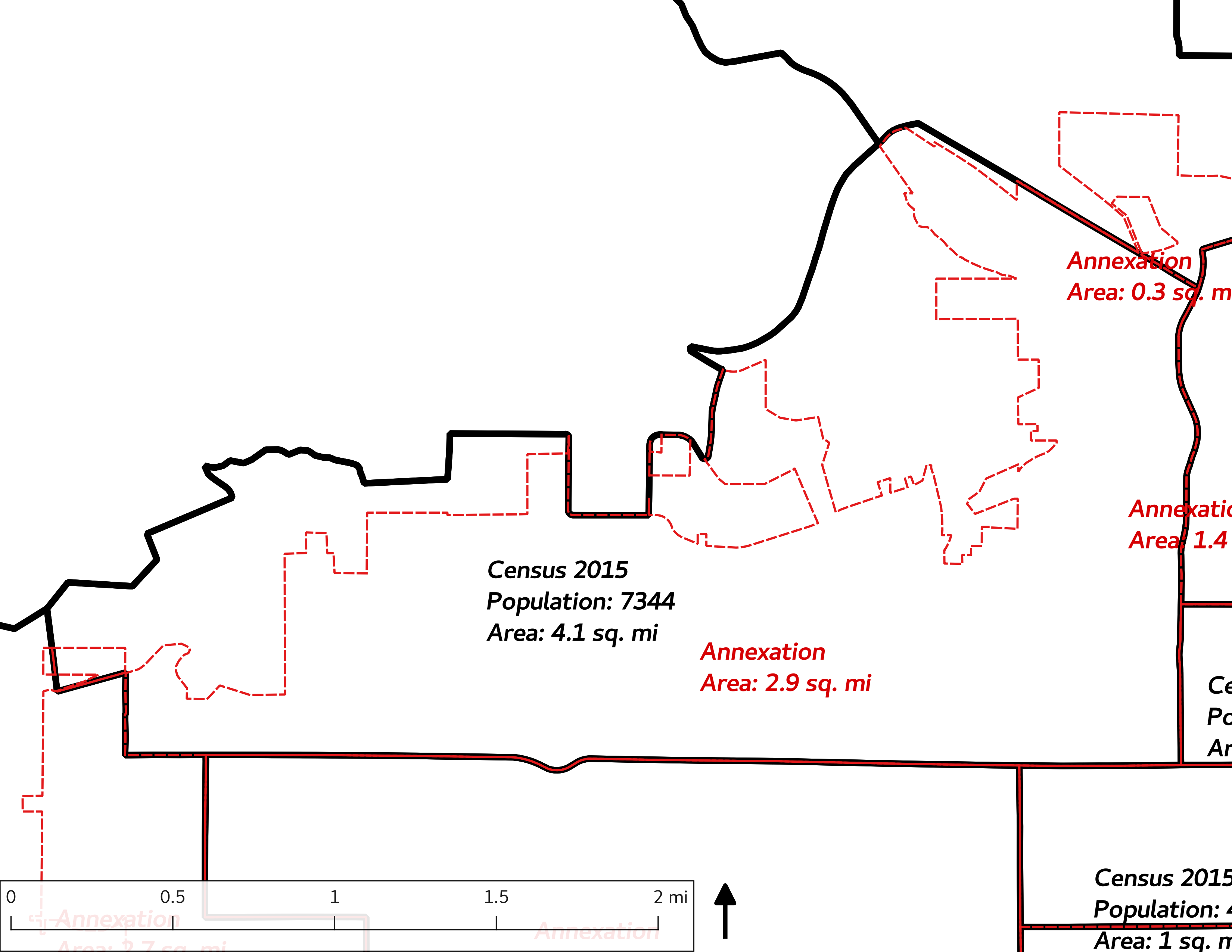
2.4.1 Historical demographics
In the first set of analyses, historical boundaries (“annexations”) of YC were overlain with contemporaneous census data to provide estimates of the demographic conditions of YC as a whole, and also stratified by the 16th Avenue dividing line. In the GIS overlay process, census tracts that are straddled by the city limits are “clipped.” The ratio of clipped to original area gives a value that can be multiplied by the original census enumeration to produce an estimate of the enumeration within the clipped area (assuming a uniform distribution across the census tract). For example if a census tract had 4000 persons, and 75% of the tract was within the city limits, the estimate of the number of persons in the portion of that tract within the city limits would be 3000 (\(4000 \times 0.75 = 3000\)). For enumerated variables (i.e., counts of persons), the sum of these area-weighted estimates was generated.
Parcel-level data were used for historical analysis of property value and year built. Because each parcel is recorded with its year of construction and assessed value, it was possible to select parcels that were in existence at each census year. It should be noted that this analysis is not truly historical, in the sense that we did not have access to data representing parcels that were redeveloped between the original year built and the census year used for the analysis.
2.4.2 Historical infrastructure allocation
In order to perform longitudinal analysis of infrastructure data stored in the GIS, it is necessary to have GIS data sets that include variables that represent when a feature of infrastructure was created or installed. Most of the GIS data sets do not include these variables, with a few notable exceptions, that can be used for historical analysis: Parks (definitely), Police and Fire Department calls (possibly–depending on how far back the data go), Animal Control, and Code Compliance (same caveats as for PD and FD calls).
For these analyses, infrastructure data were selected to match the year of the census data, such that the GIS data selection represented those infrastructure features that existed at the time of the census. The infrastructure data were then overlain on the census data to generate tables in support of statistical analysis comparing potential infrastructure accessibility and demographic patterns.
2.4.2.1 Parks
Historical analysis of parks was done using two separate methods. For both methods, two runs were made, (1) incuding all parks, and (2) excluding any parks that had received any private funding:
- CHESTERLEY PARK
- FRANKLIN PARK & POOL
- HARMAN CENTER AT GAILLEON PARK
- KIWANIS PARK & GATEWAY SPORTS COMPLEX
- LARSON PARK
- MILLER PARK
- NORTH 44TH AVE PARK
- RANDALL PARK
- ROSALMA GARDEN CLUB PARK
- SOUTHEAST COMMUNITY PARK
2.4.2.1.1 Overlay of parks with census tracts
For both data sets, years were matched (e.g., for the 1980 census, only those parks that existed in 1980 were selected). A GIS intersection was performed to tabulate the total area of parks within each census tract. Demographic characteristics of the tract and the area of parks within the tract were graphed as scatter plots.
2.4.2.1.2 Buffer of park polygons by 1/4 mile
Buffers of 1/4 mile, as a proxy for locations within reasonable walking distance, were generated for the parks polygons; these buffers were then overlain on the census tracts to obtain estimated demographic counts within and outside the buffers. The relative proportion of persons in each demographic category were tabulated using the same year-to-year matching.
2.4.2.1.3 Stratification by 16th Avenue
Total area of parks per capita was tabulated for each year with stratification by 16th Avenue.
2.4.3 Current infrastructure/services allocation
Most of the GIS data sets are not encoded for historical analysis. To be used for historical analysis, each feature in each layer would require an attribute value representing the year in which the infrastructure feature was installed or created (this is not to be confused with the date in which a feature was added to a GIS layer). This is not a requirement for urban GIS, which typically is updated with new data to create a layer representing current conditions. Having historical data in the YC GIS would have required a decision to be made at the system’s initiation to store these dates.
2.4.3.1 Public safety calls for service
Yakima Fire and Police Department calls for service were tallied at the census tract level, normalized by the census count of persons per tract (i.e., resulting in the number of calls per person). Response times were not provided and were not available for any of the public safety calls for service.
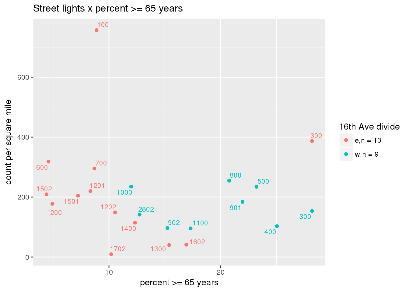
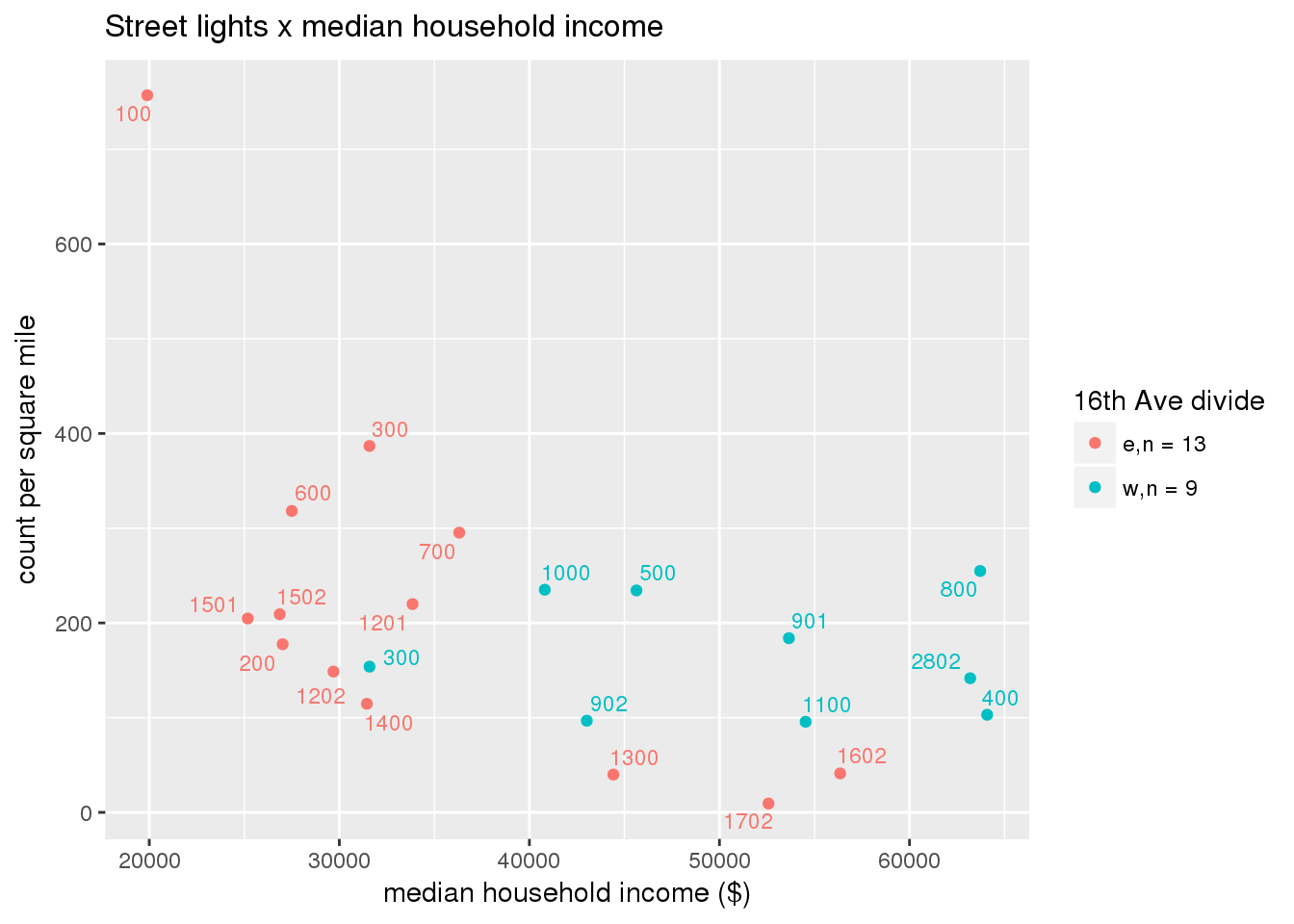
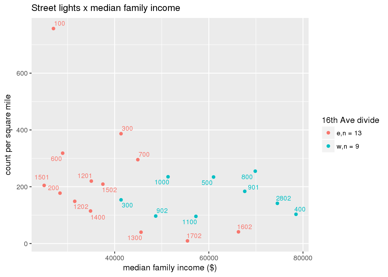
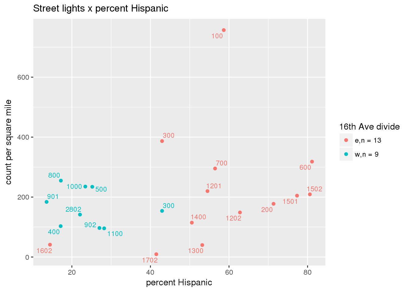
2.4.3.2 Street lights
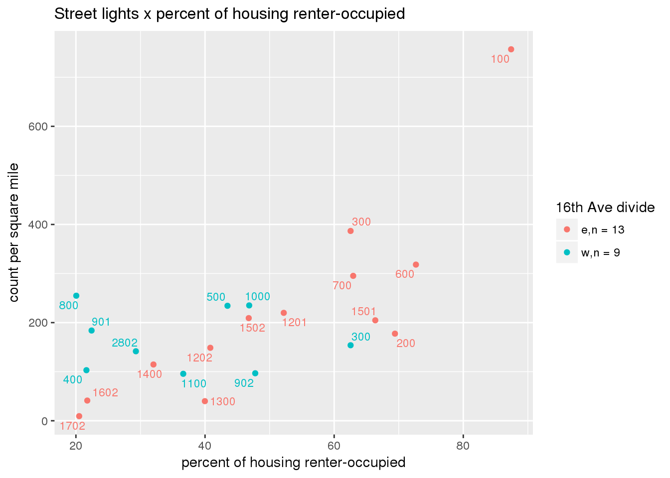
Street lights were tallied at the census tract level, normalized by the tract area (i.e., resulting in the number of street lights per unit area).
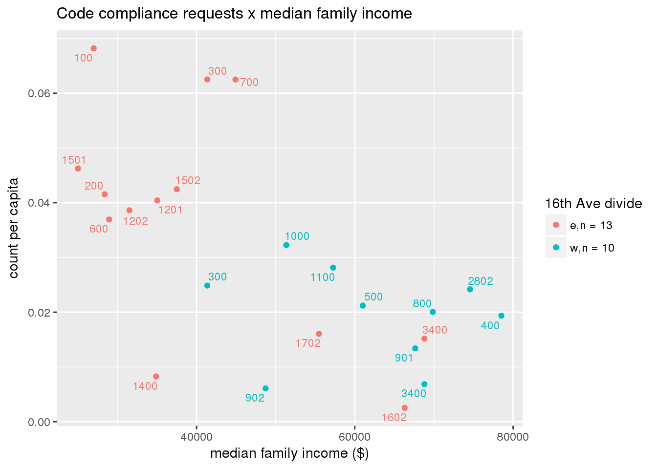
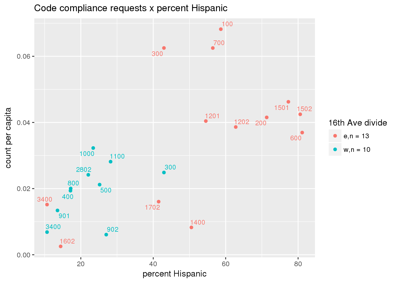
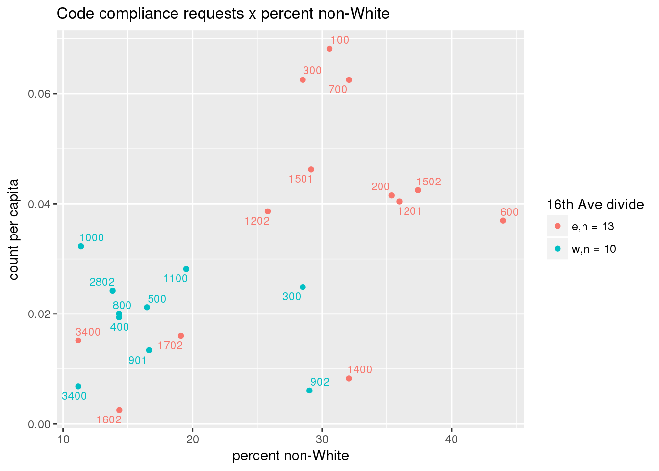
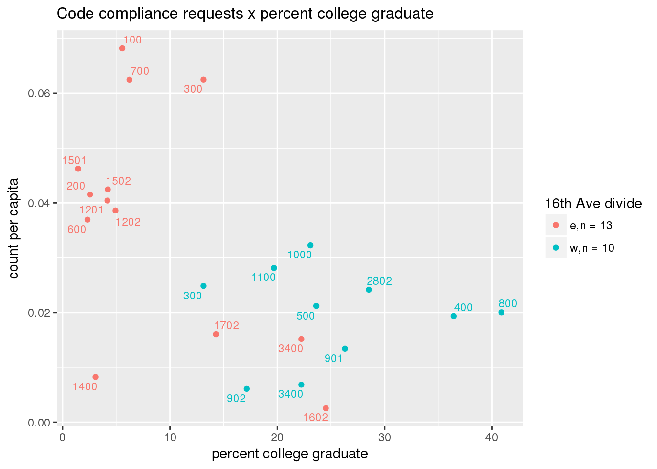
2.4.3.3 Code compliance requests
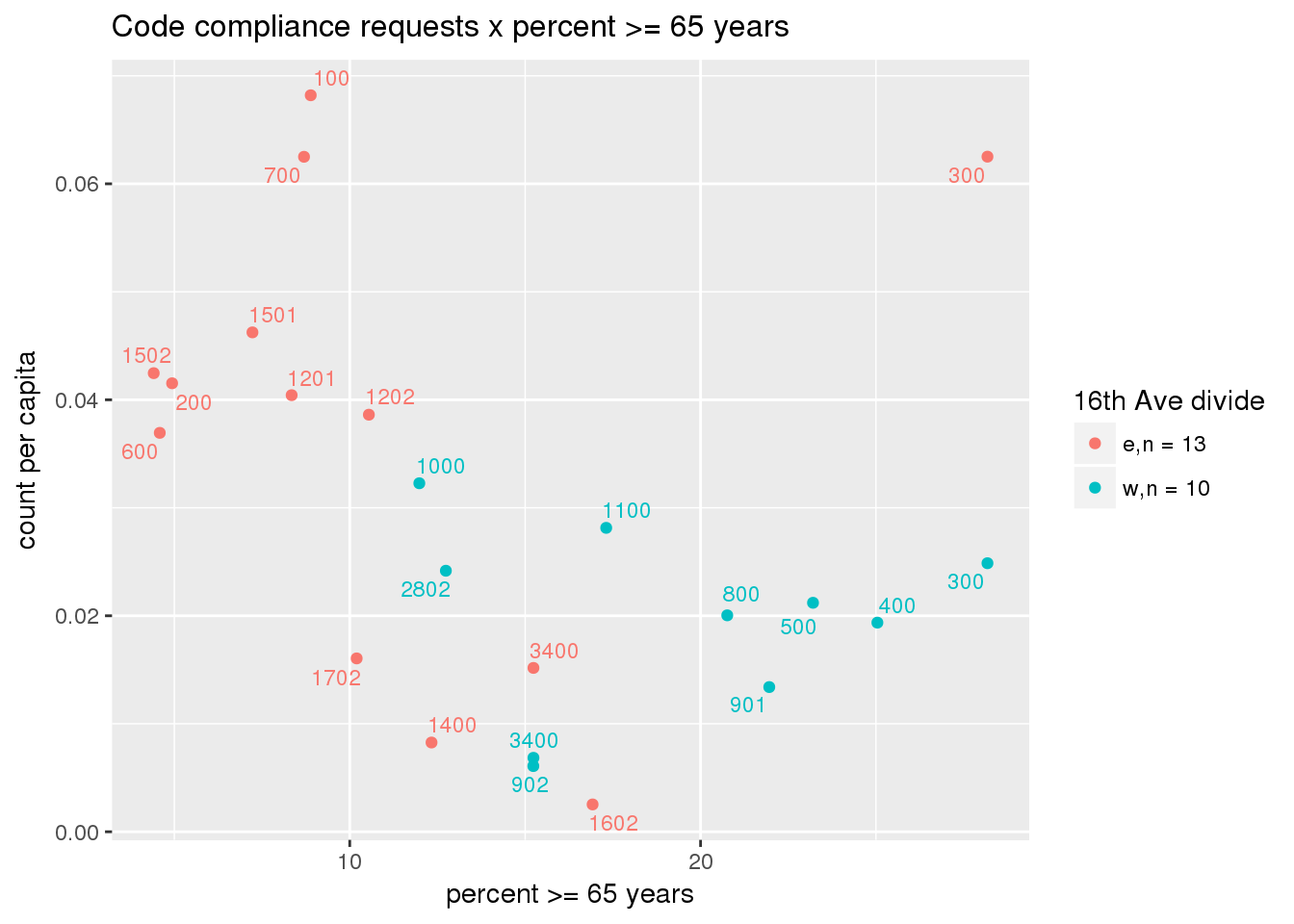
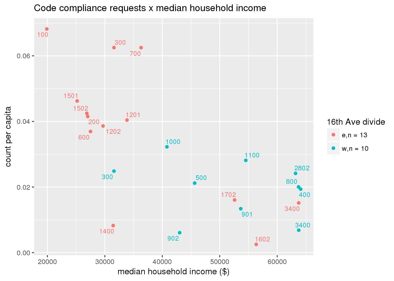
Code compliance requests were treated in the same manner as public safety calls (i.e., calls per capita).
2.4.3.4 Transit
Transit data were analyzed similarly, using density of counts of ridership, benches, and shelters per capita.
3 Results
Results are presented for each selected GIS data layer and demographic variable.
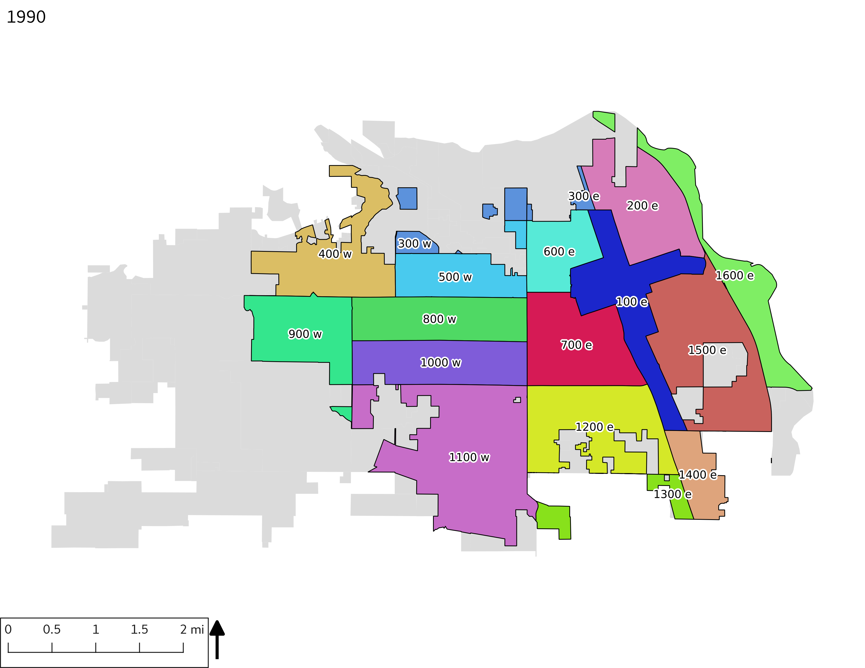
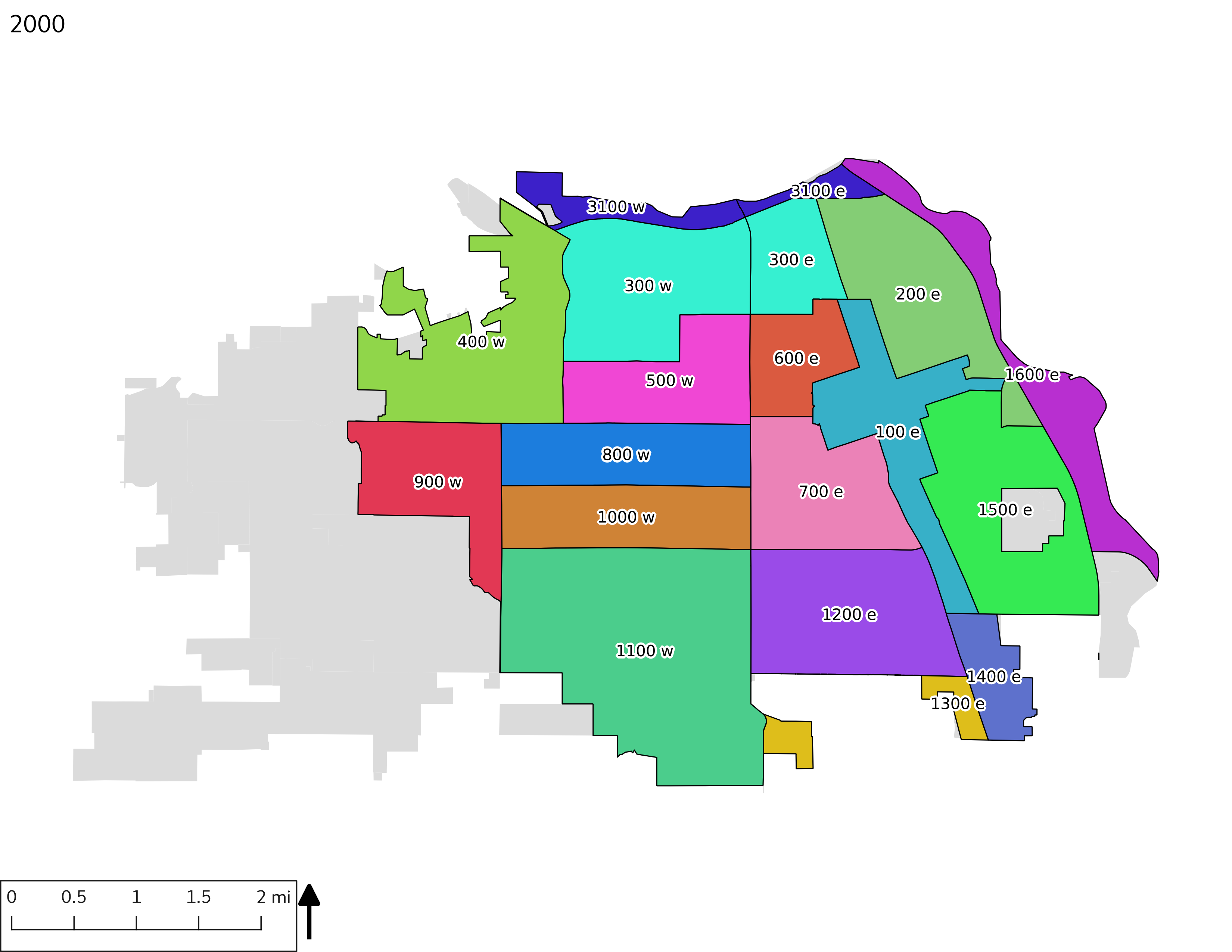
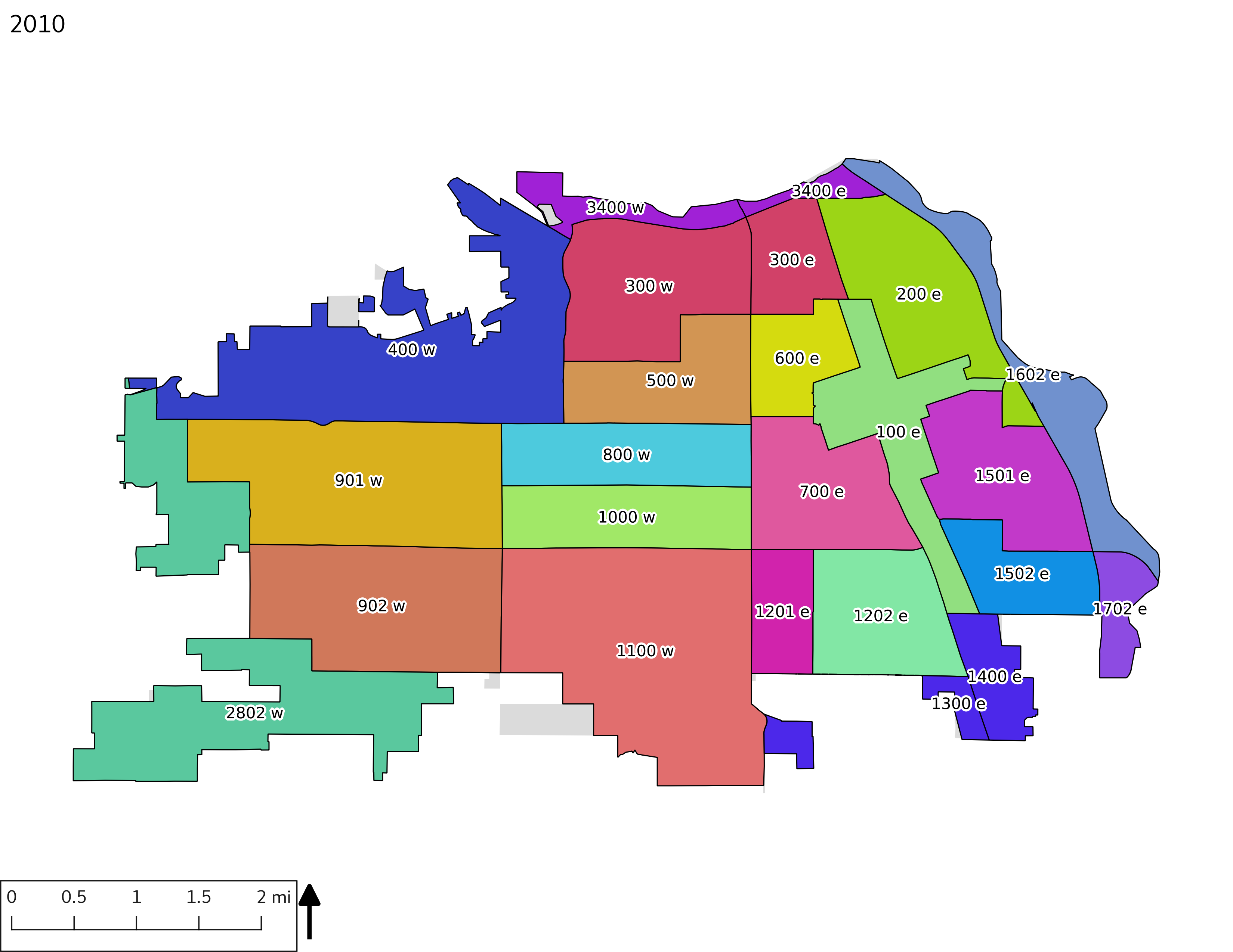
3.1 Census tract population
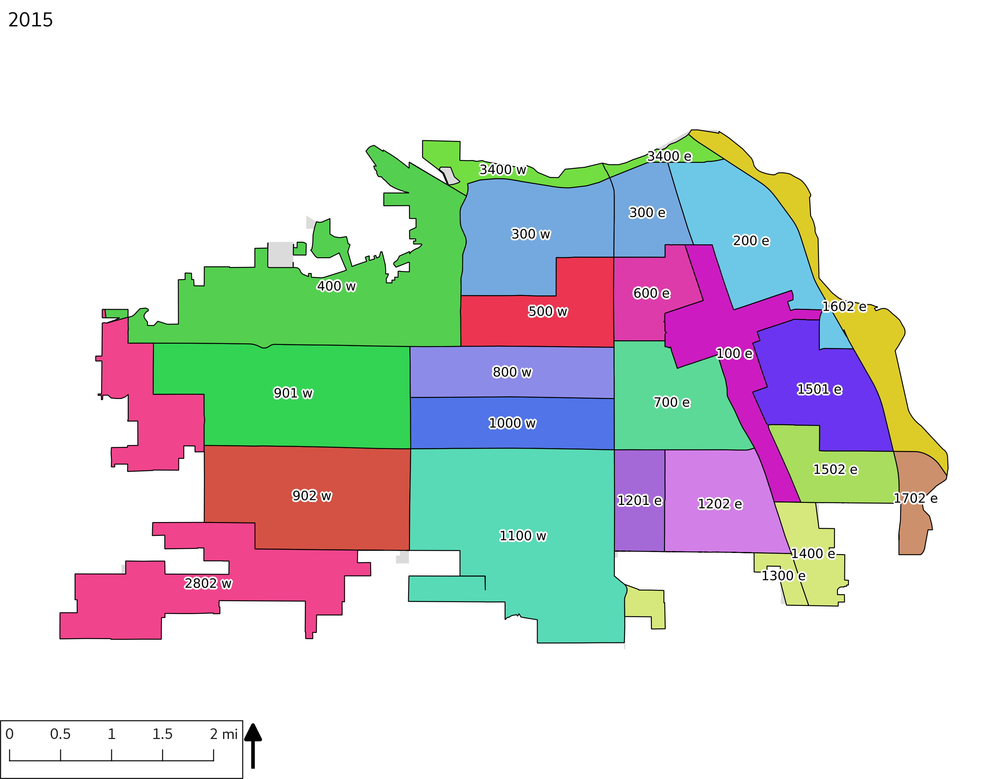
To aid in interpretation of the demographic graphs, the following table and set of maps enumerate census tracts with population (in the table) and tract IDs (in the table and on the maps). The tract IDs can be used to cross-reference the graphs and the maps. It should be noted that some tract IDs changed over time, such as tract 900 being split to 901 and 902 after the year 2000, and some tracts had no overlap with the city limits in earlier years (e.g., 2802).
censuspop <- dbGetQuery(conn = us_census, statement = "with
                                y1980 as (select right(tract::text, 4)::int as tract, round(sum(total_pop)::numeric,0) as pop_1980 from yakima_equity.tract_1980 group by tract)
                                , y1990 as (select right(tract::text, 4)::int as tract, round(sum(total_pop)::numeric,0) as pop_1990 from yakima_equity.tract_1990 group by tract)
                                , y2000 as (select right(tract::text, 4)::int as tract, round(sum(total_pop)::numeric,0) as pop_2000 from yakima_equity.tract_2000 group by tract)
                                , y2010 as (select right(tract::text, 4)::int as tract, round(sum(total_pop)::numeric,0) as pop_2010 from yakima_equity.tract_2010 group by tract)
                                , y2015 as (select right(tract::text, 4)::int as tract, round(sum(total_pop)::numeric,0) as pop_2015 from yakima_equity.tract_2015 group by tract)
                                , f as (select * from y1980 full join y1990 using (tract) full join y2000 using (tract) full join y2010 using (tract) full join y2015 using (tract))
                                select tract::numeric, pop_1980, pop_1990, pop_2000, pop_2010, pop_2015 from f order by tract;")

                                census_descr_cap <- table_nums(name="census_descr_cap", caption = "Estimated census tract population over time")
kable(censuspop, format = "html", caption = census_descr_cap)| tract | pop_1980 | pop_1990 | pop_2000 | pop_2010 | pop_2015 |
|---|---|---|---|---|---|
| 100 | 2113 | 2426 | 2778 | 3356 | 3094 |
| 200 | 3221 | 3665 | 5374 | 5787 | 5996 |
| 300 | 232 | 493 | 3905 | 4172 | 4216 |
| 400 | 1635 | 1719 | 2758 | 5011 | 5216 |
| 500 | 3327 | 3730 | 5011 | 5811 | 5141 |
| 600 | 3829 | 4566 | 6485 | 6866 | 7743 |
| 700 | 5995 | 6447 | 6684 | 6477 | 7520 |
| 800 | 5086 | 4822 | 4614 | 4398 | 4441 |
| 900 | 1325 | 1830 | 2596 | NA | NA |
| 901 | NA | NA | NA | 7504 | 7464 |
| 902 | NA | NA | NA | 3341 | 4110 |
| 1000 | 5459 | 5689 | 5725 | 5541 | 5516 |
| 1100 | 2244 | 2749 | 4065 | 4460 | 4691 |
| 1200 | 5932 | 6509 | 9048 | NA | NA |
| 1201 | NA | NA | NA | 3712 | 3859 |
| 1202 | NA | NA | NA | 6415 | 6344 |
| 1300 | 187 | 178 | 197 | 219 | 194 |
| 1400 | 630 | 591 | 660 | 674 | 726 |
| 1500 | 2841 | 6583 | 8380 | NA | NA |
| 1501 | NA | NA | NA | 6132 | 7569 |
| 1502 | NA | NA | NA | 2616 | 2944 |
| 1600 | 42 | 154 | 215 | NA | NA |
| 1602 | NA | NA | NA | 764 | 791 |
| 1702 | NA | NA | NA | 64 | 62 |
| 2802 | NA | NA | NA | 1784 | 1903 |
| 3100 | NA | NA | 123 | NA | NA |
| 3400 | NA | NA | NA | 182 | 212 |
3.1.1 Census tract maps
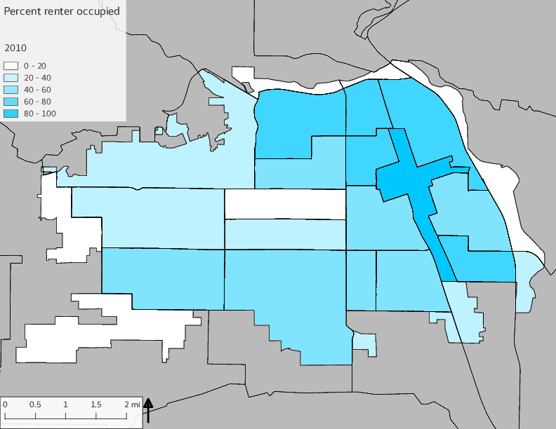
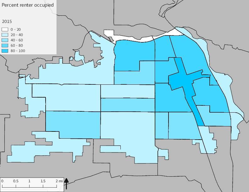
The set of Census tract maps display the census tracts with census tract identifier and “e” or “w” based on the 16th Avenue dividing line. These maps, along with the tables of Census tract demographic aggregates should be helpful in interpreting the scatter plots, which include text labels showing the tract identifiers. It should be noted that 16th Avenue divides some tracts; for those tracts that span 16th Avenue, there will be two data points on the map, each with an area-weighted estimate of the proportion of the both X and Y variables.
include_graphics(tractmaps)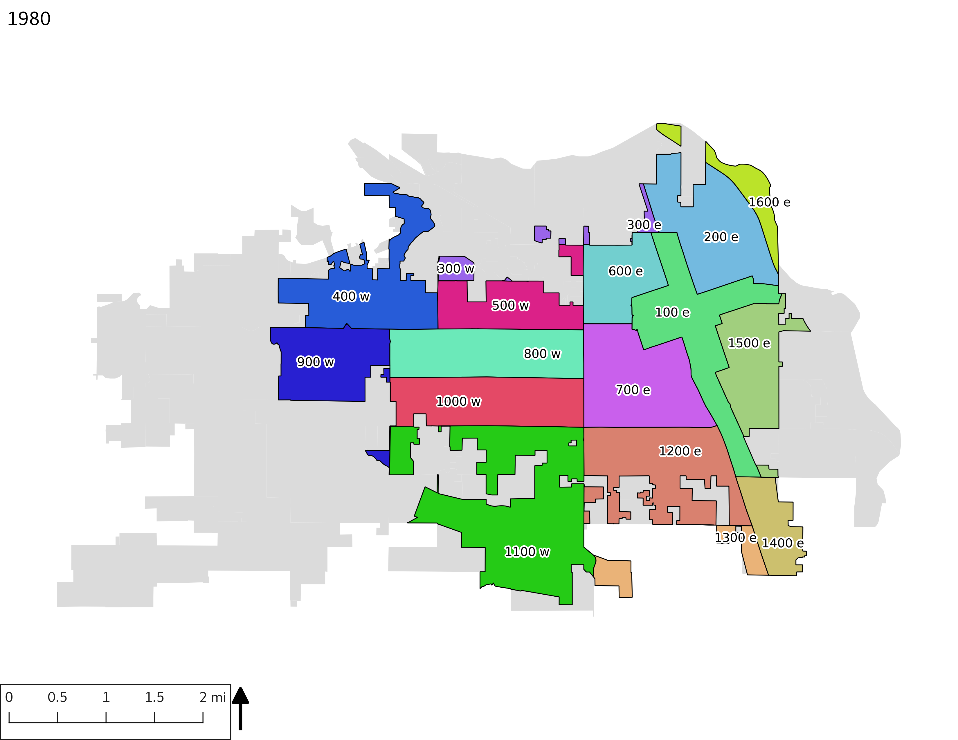
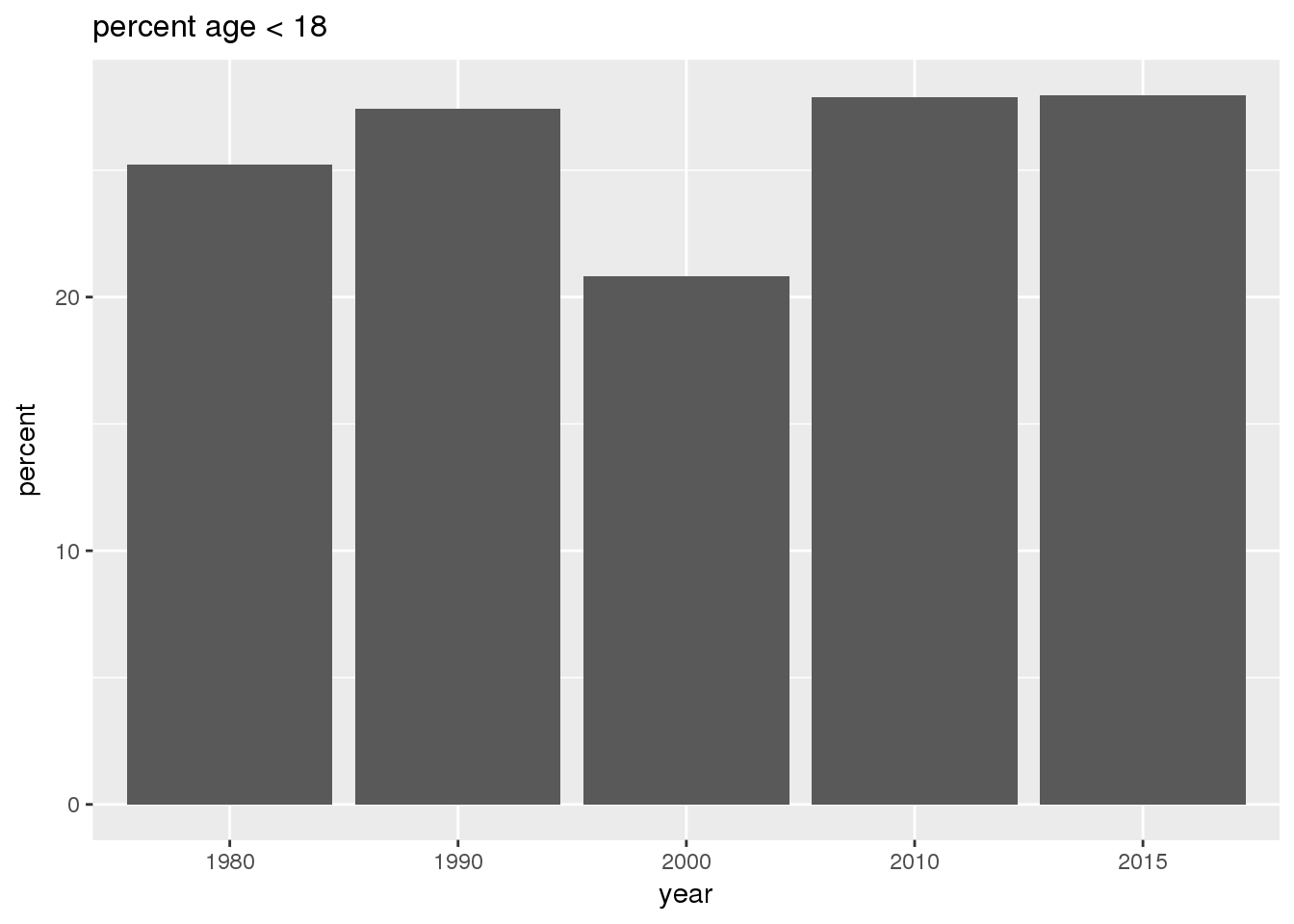
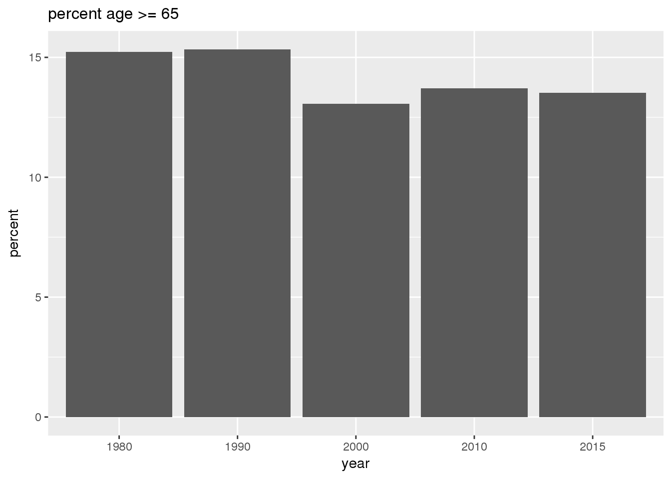
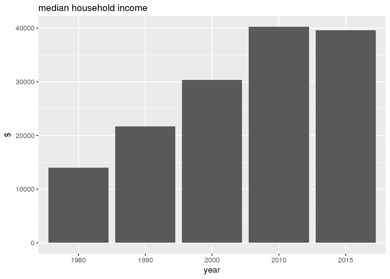
3.2 Historical demograpics
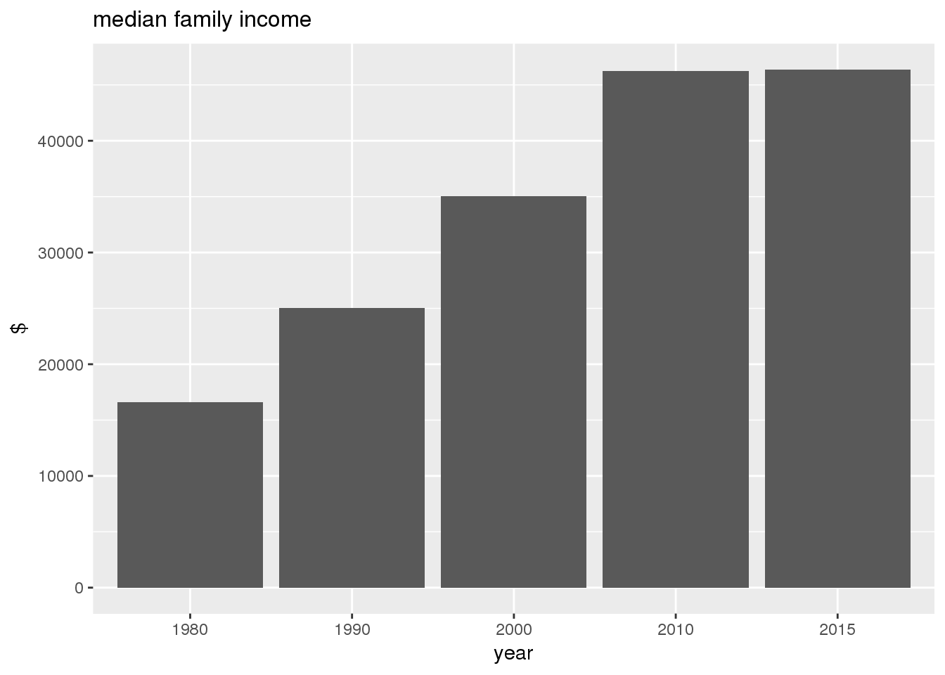
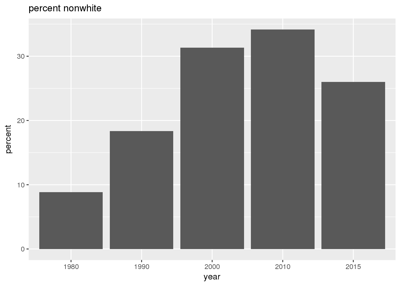
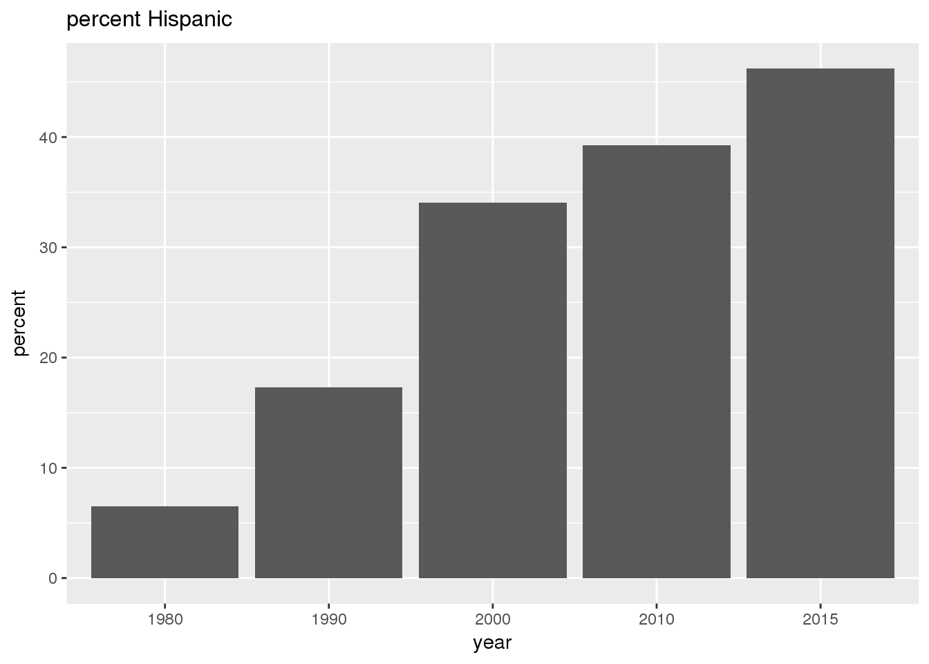
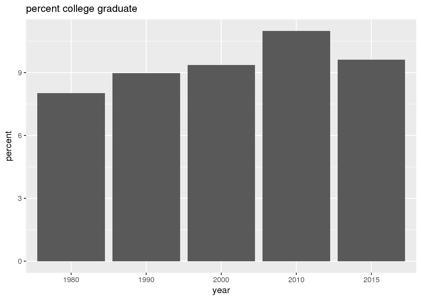
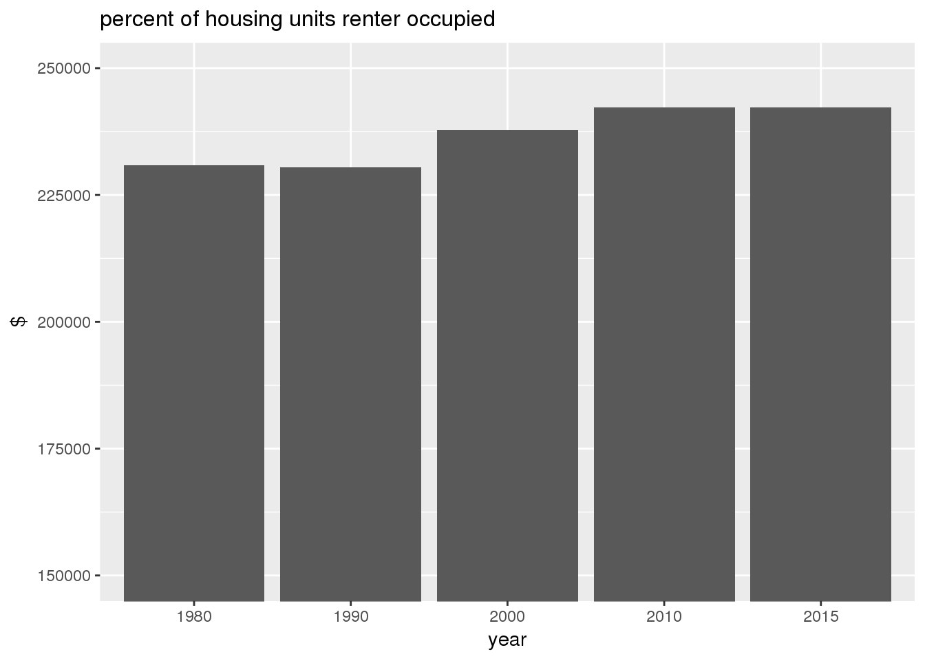
3.2.1 City of Yakima as a whole
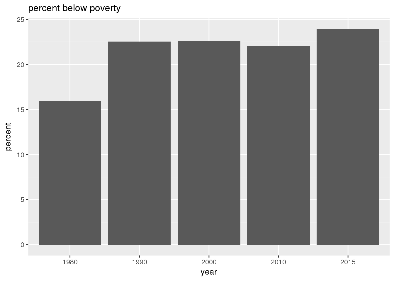
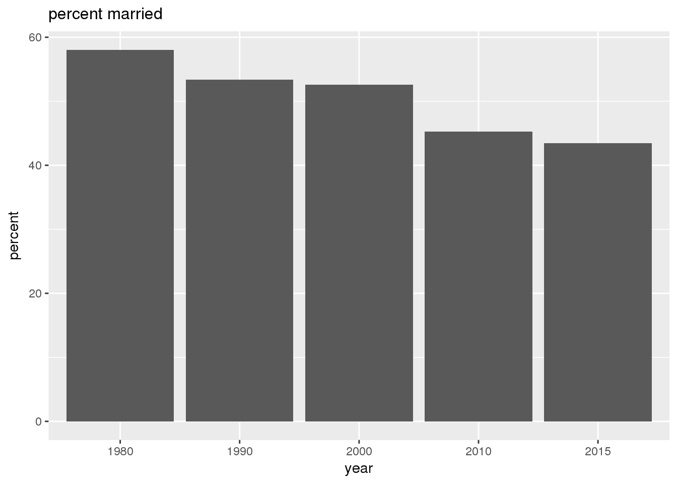
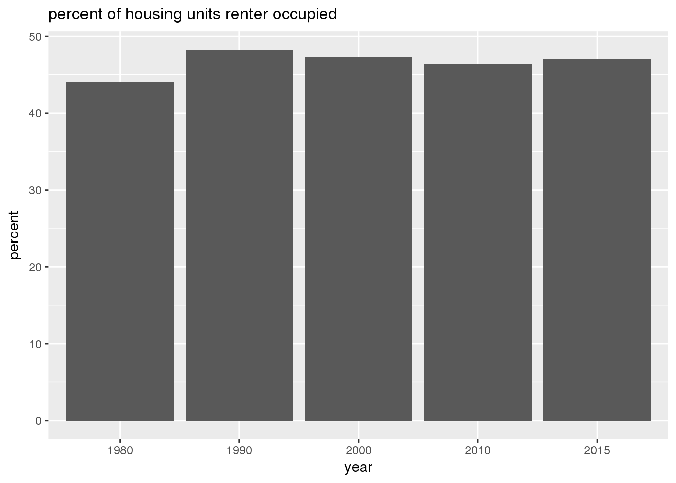
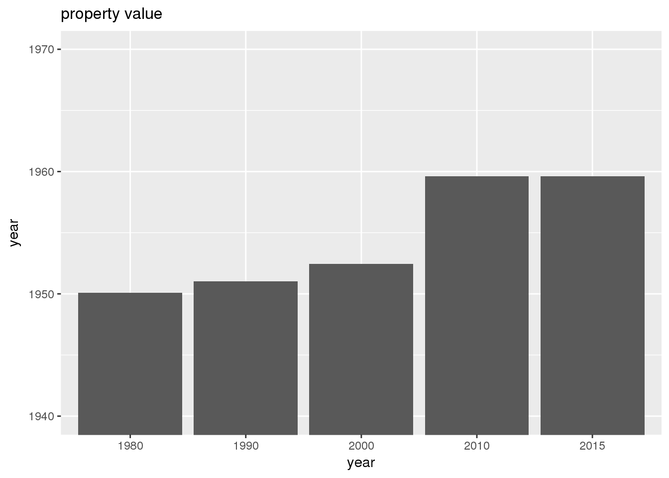
The graphs show in bar graphs the same set of demographic variables over time that were shown in the maps. However, the graphs show aggregate values for the entire city in this section and . Bars represent numerical quantities (i.e., percent of population, USD, year) on the y-axis, and years are indexed on the x-axis.
# Creates materialized views of median property value and mean year built per tract bsaed on parcel level data
                                    sql <- "drop materialized view if exists yakima_equity.tract_propval_xxxYEARxxx cascade;
                                    create materialized view yakima_equity.tract_propval_xxxYEARxxx as
                                    with
                                    --tracts
                                    t as (select * from yakima_equity.tract_xxxYEARxxx)
                                    --parcels
                                    , p as (select tract, mkt_land + mkt_impvt as propvalue, year_blt::integer from yakima_equity.parcels as p, t where st_intersects(st_centroid(p.the_geom_2286), t.the_geom_2286) and year_blt::integer <= xxxYEARxxx and mkt_land > 0 and mkt_impvt > 0)
                                    --median value and mean year built
                                    , m as (select tract, PERCENTILE_CONT(0.50) WITHIN GROUP (ORDER BY propvalue)::integer AS median_propvalue, avg(year_blt)::integer as mean_year_built from p group by tract)
                                    --join back to tract
                                    , j as (select row_number() over() as gid, tract, St_Multi(the_geom_2286)::geometry(MultiPolygon, 2286) as geom, median_propvalue, mean_year_built from t join m using(tract))
                                    select * from j;"

                                    for(i in years){
                                        sqli <- gsub("xxxYEARxxx", i, sql)
                                        O <- dbGetQuery(conn = dbconn, statement = sqli)
                                    }

                                    citysum <- ycsum.all(zone = FALSE)
                                    # column names to titles
                                    citysum <- sqldf("select year, pct_age_lt_18, pct_age_ge_65, median_hh_income, median_family_income, pct_nonwhite, pct_hispanic, pct_edu_coll_grad, pct_pov_below_100pct, pct_married, pct_housingunits_renter, propvalue, year_built from citysum")
                                    titles <- c("year", "percent age < 18", "percent age >= 65", "median household income", "median family income", "percent nonwhite", "percent Hispanic", "percent college graduate", "percent below poverty", "percent married", "percent of housing units renter occupied", "property value", "mean year built")
                                    for(i in 2:(ncol(citysum) - 2)){
                                        colname <- colnames(citysum)[i]
                                        title <- titles[i]
                                        ylab <- switch(substr(colname, 1, 3),
                                            med="$",
                                            pct="percent",
                                            pro="$",
                                            yea="year")

                                        g <- ggplot(data = citysum, aes(factor(year), citysum[,i])) + geom_bar(stat = "identity") + labs(x="year", y=ylab, title=title) +
                                        theme(plot.title = element_text(size=12))

                                        if(colname=='year_built'){
                                            g <- g + coord_cartesian(ylim = c(1940, 1970))
                                        }
                                        if(colname=='propvalue'){
                                            g <- g + coord_cartesian(ylim = c(150000, 250000))
                                        }
                                        print(g)
                                        ggsave(filename = file.path(imagedir, sprintf("%s.png", colname)), plot = g, width = ggsavewidth, height = ggsaveheight, units = "in")
                                    }
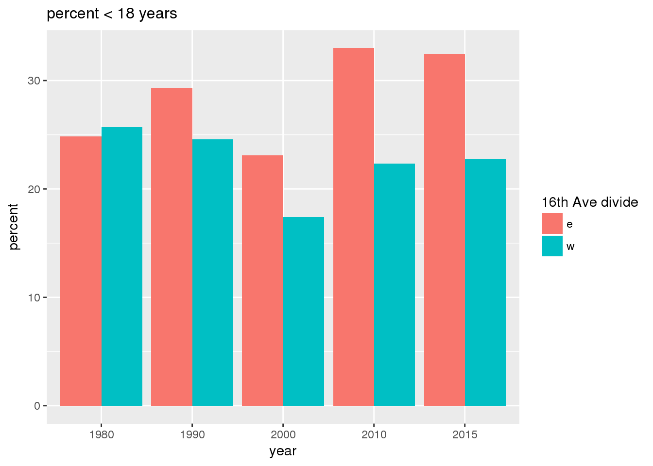
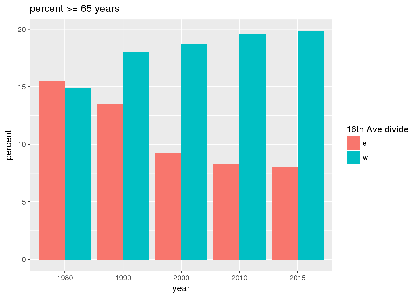
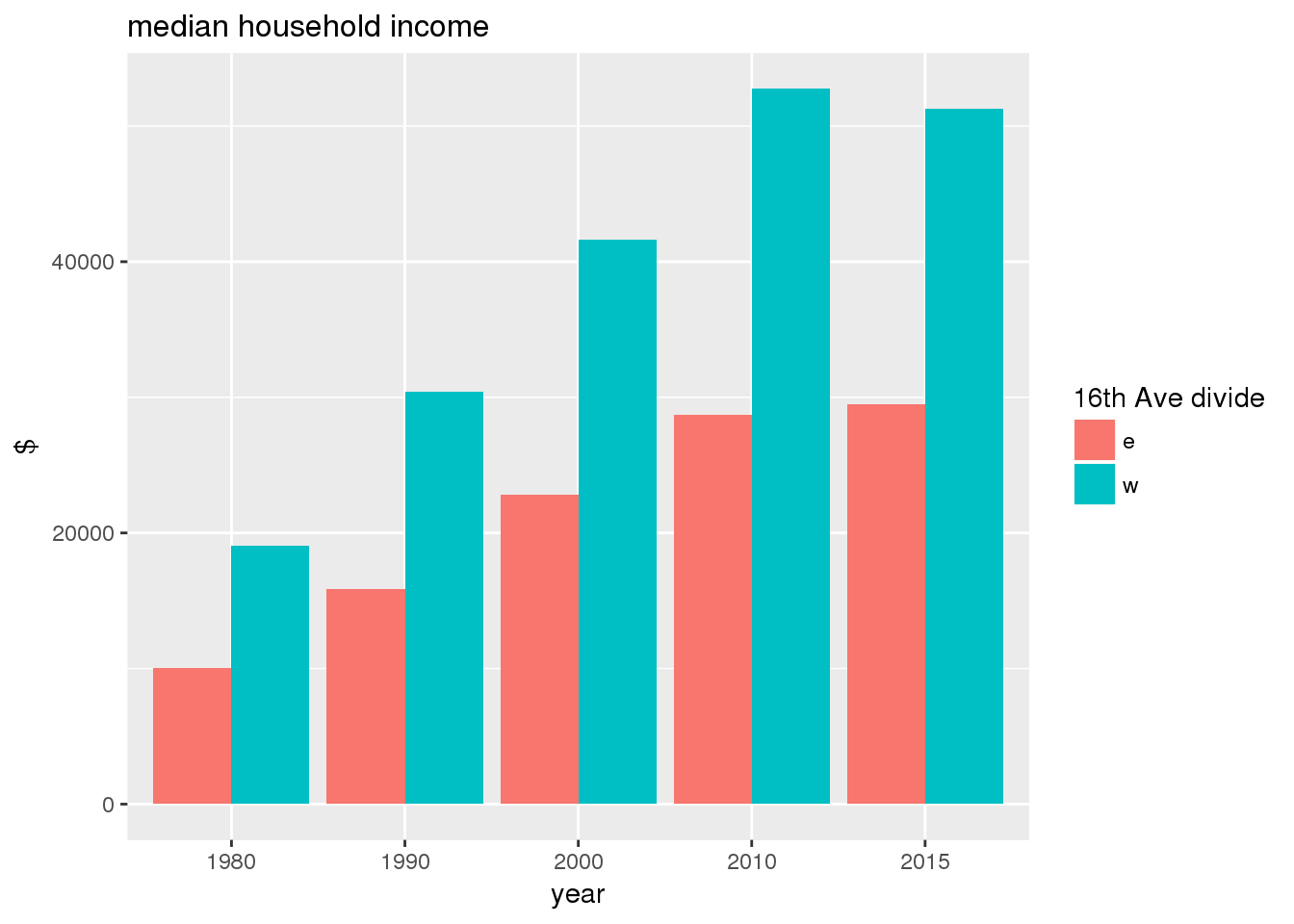
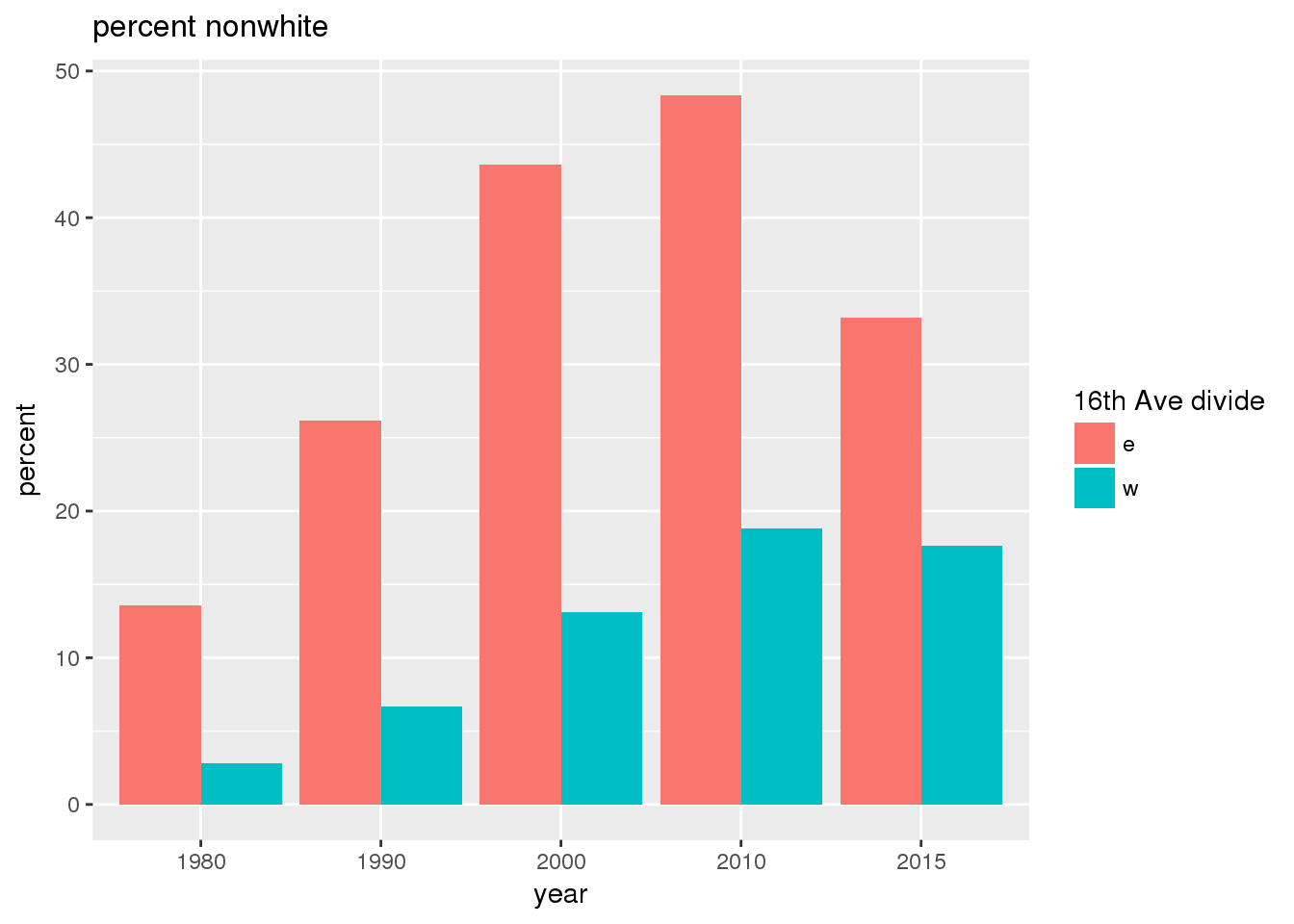
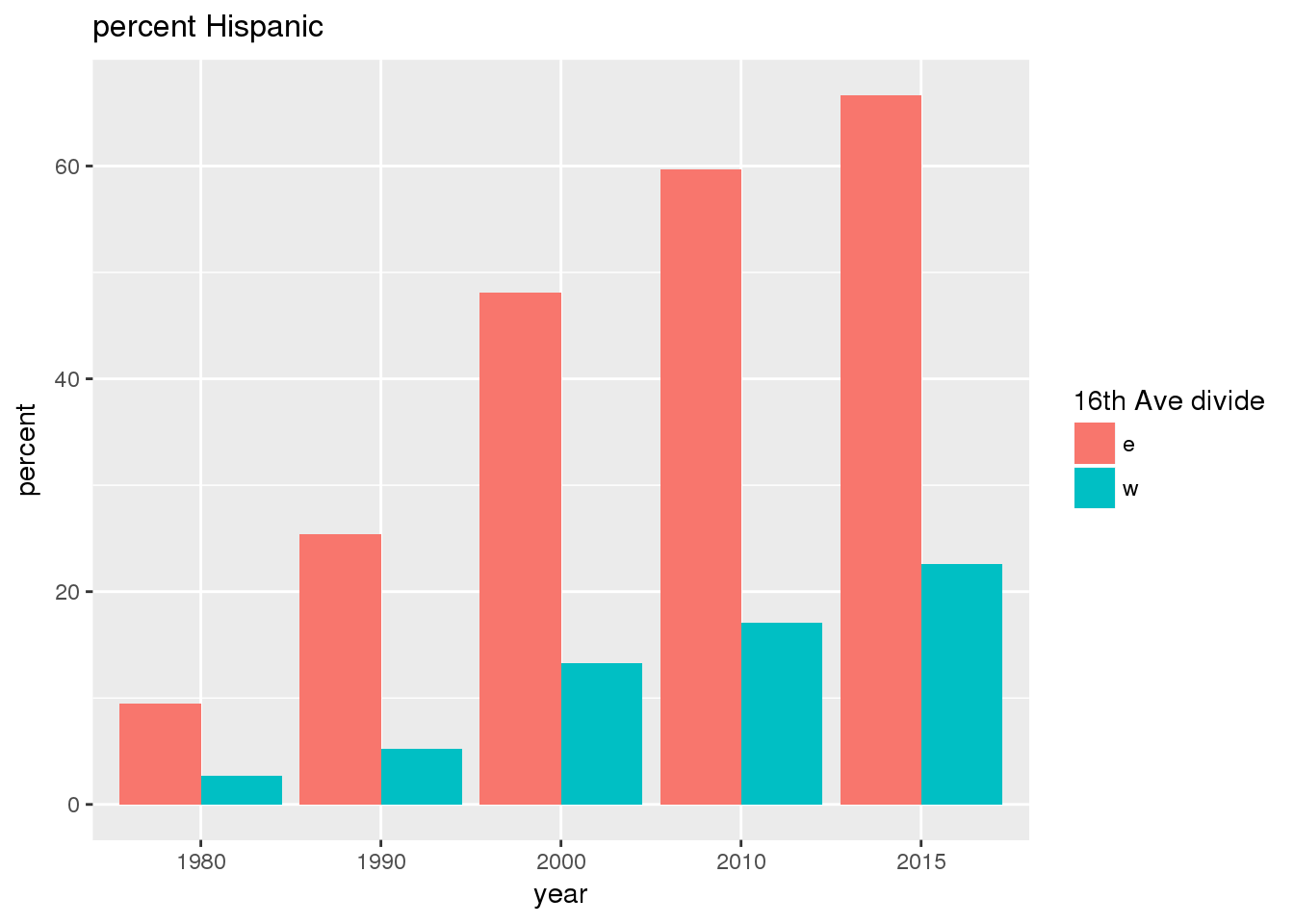
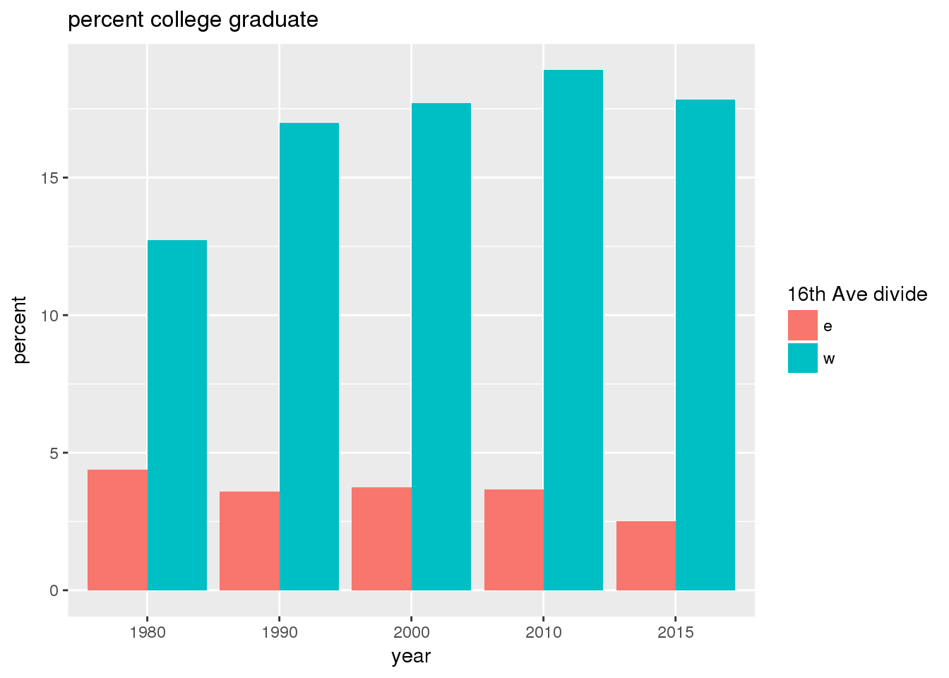
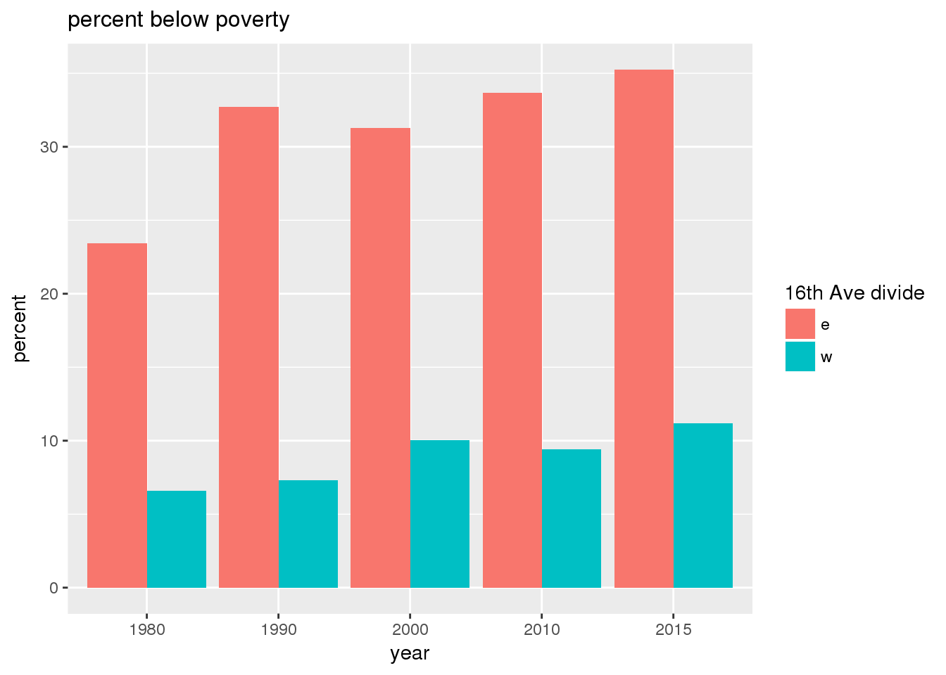
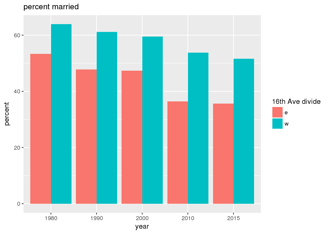
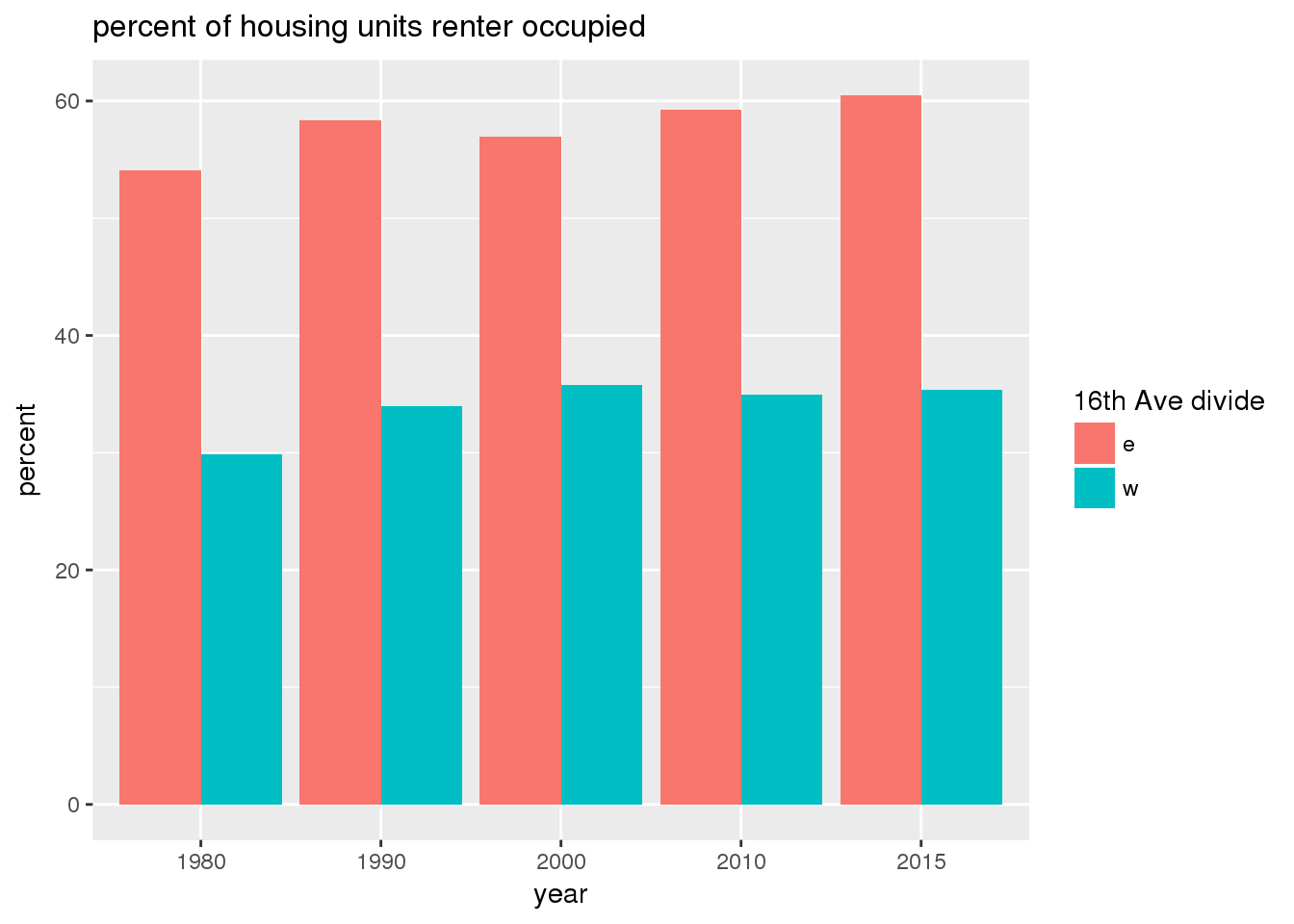
3.2.2 Sixteenth Avenue stratification
This section includes the same set of graphs as above, but stratified by 16th Avenue. Bars in one color represent the quantities on the east side, and the other color represents quantities on the west side.
ewsum <- ycsum.all(zone = TRUE)
                                    ewsum <- sqldf("select zone_16th, year, pct_age_lt_18, pct_age_ge_65, median_hh_income, median_family_income, pct_nonwhite, pct_hispanic, pct_edu_coll_grad, pct_pov_below_100pct, pct_married, pct_housingunits_renter, propvalue, year_built from ewsum")
                                    titles <- c("zone", "year", "percent < 18 years", "percent >= 65 years", "median household income", "median family income", "percent nonwhite", "percent Hispanic", "percent college graduate", "percent below poverty", "percent married", "percent of housing units renter occupied", "property value", "year built")
                                    for(i in 3:(ncol(ewsum)-2)){
                                        colname <- colnames(ewsum)[i]
                                        title <- titles[i]
                                        ylab <- switch(substr(colname, 1, 3),
                                        med="$",
                                        pct="percent",
                                        pro="$",
                                        yea="year")

                                        g <- ggplot(data = ewsum, aes(factor(year), ewsum[,i], fill=zone_16th)) + geom_bar(stat = "identity", position = "dodge") + labs(x="year", y=ylab, title=title, fill="16th Ave divide") +
                                        theme(plot.title = element_text(size=12))

                                        if(colname=='year_built'){
                                            g <- g + coord_cartesian(ylim = c(1940, 1970))
                                        }
                                        if(colname=='propvalue'){
                                            g <- g + coord_cartesian(ylim = c(150000, 250000))
                                        }
                                        print(g)
                                        ggsave(filename = file.path(imagedir, sprintf("%s_16th.png", colname)), plot = g, width = ggsavewidth, height = ggsaveheight, units = "in")

                                }

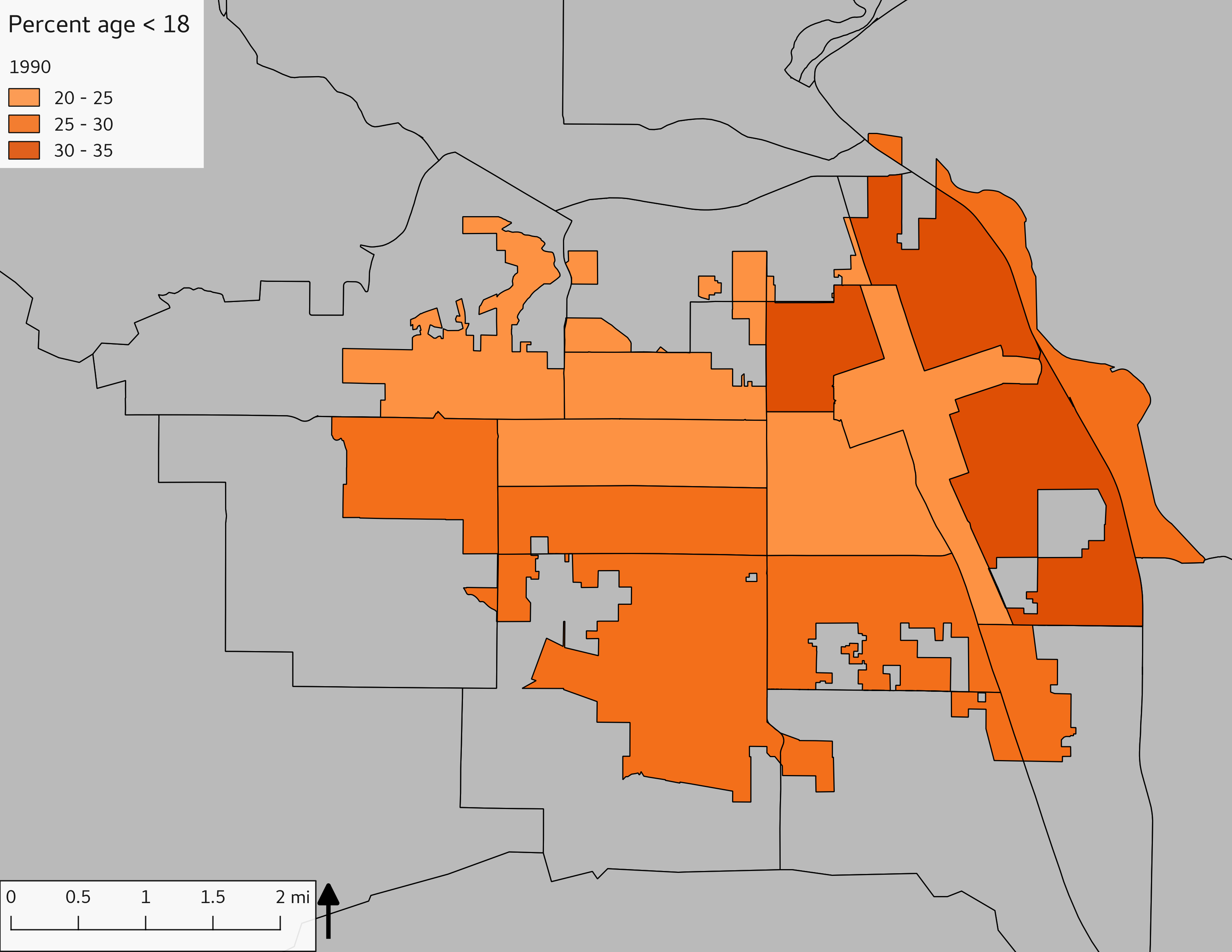
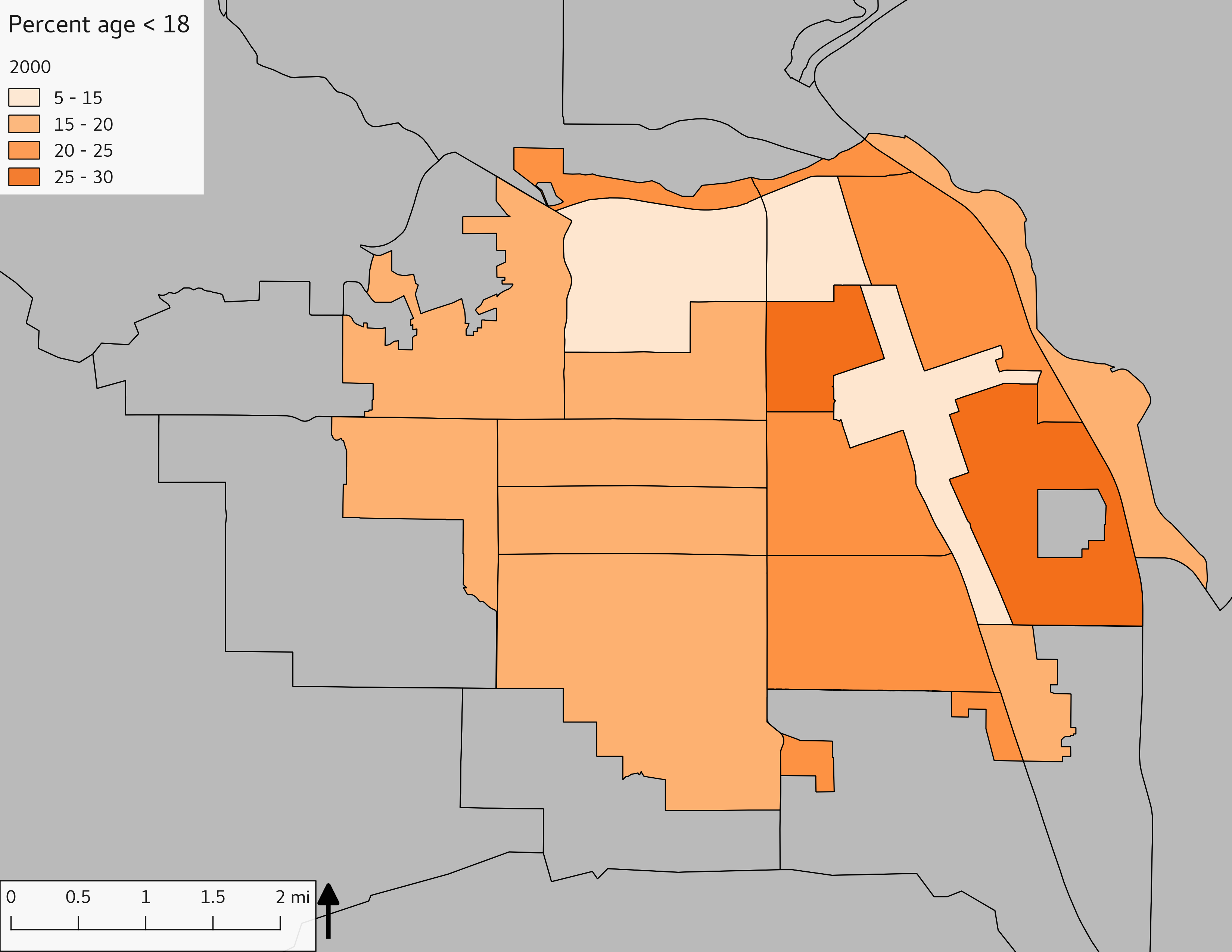
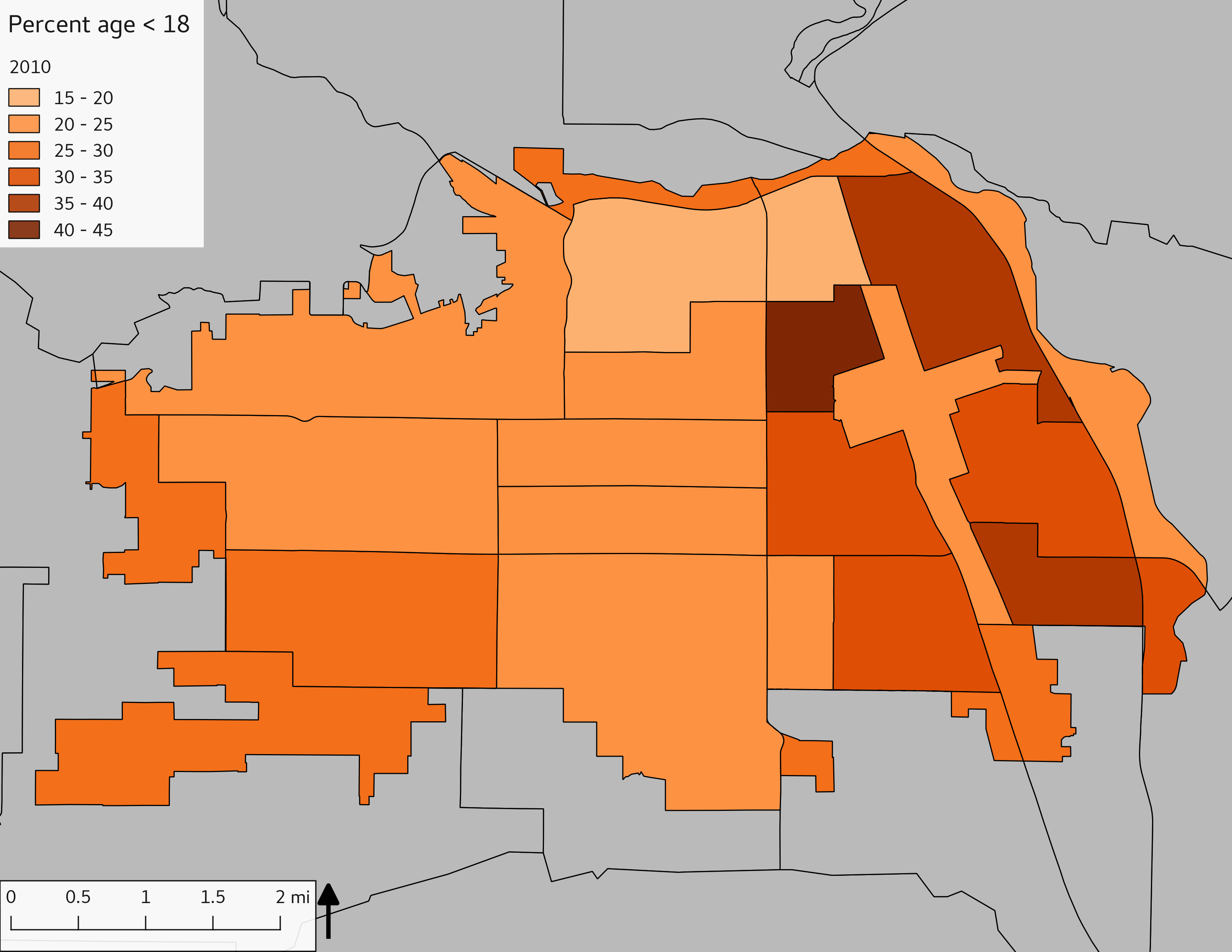
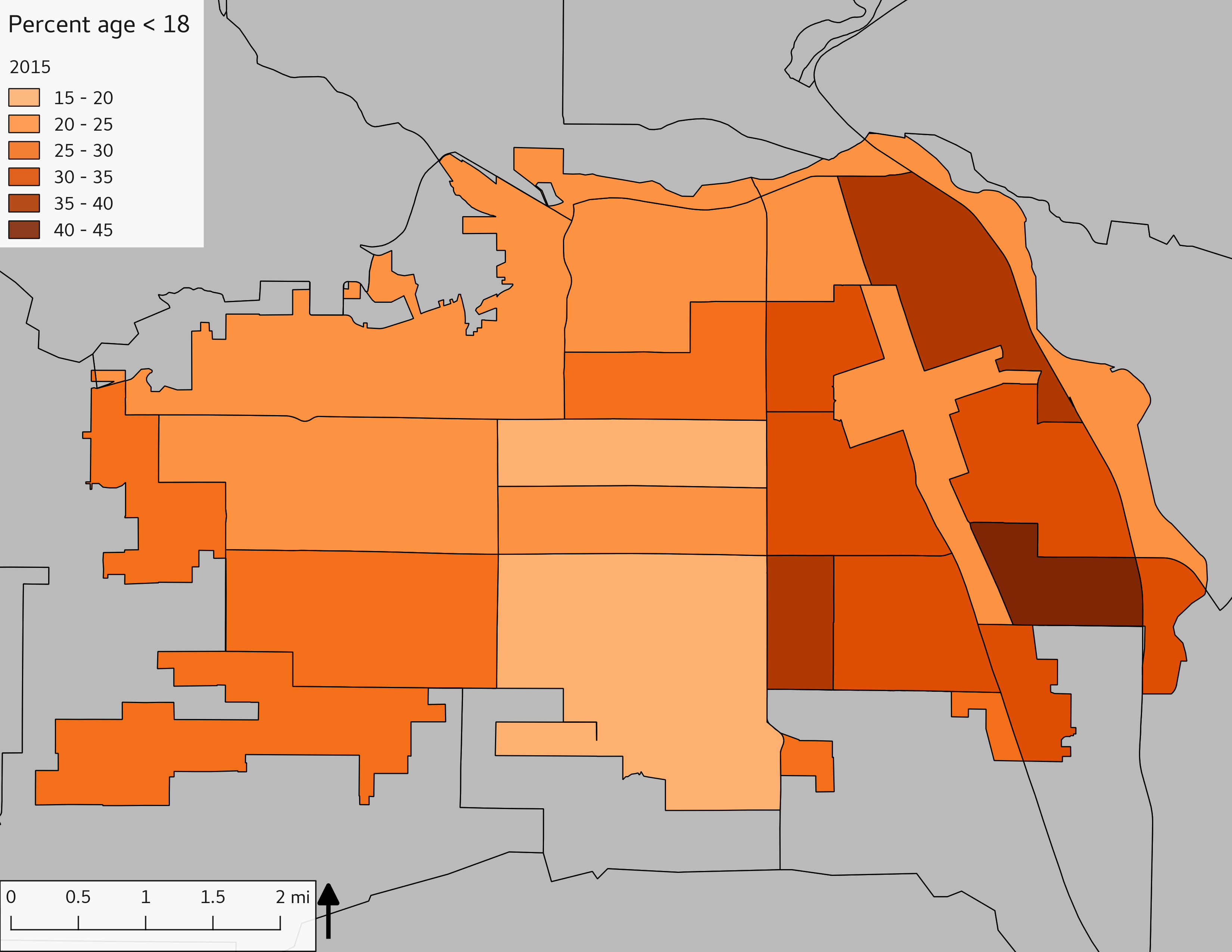
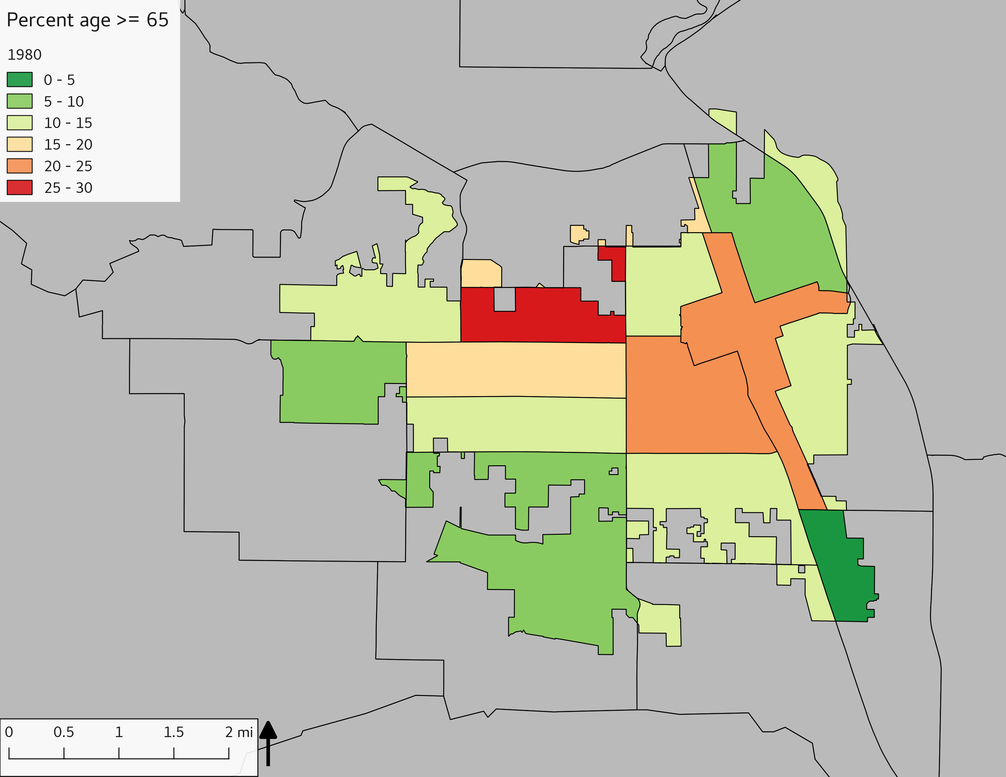
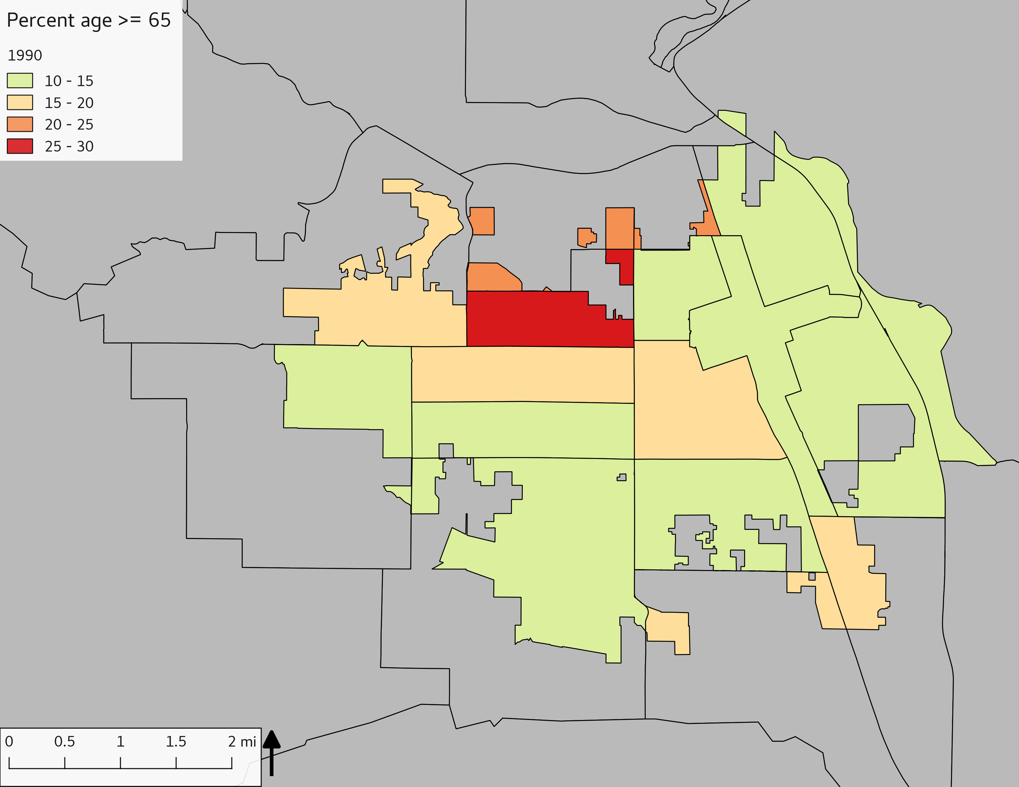
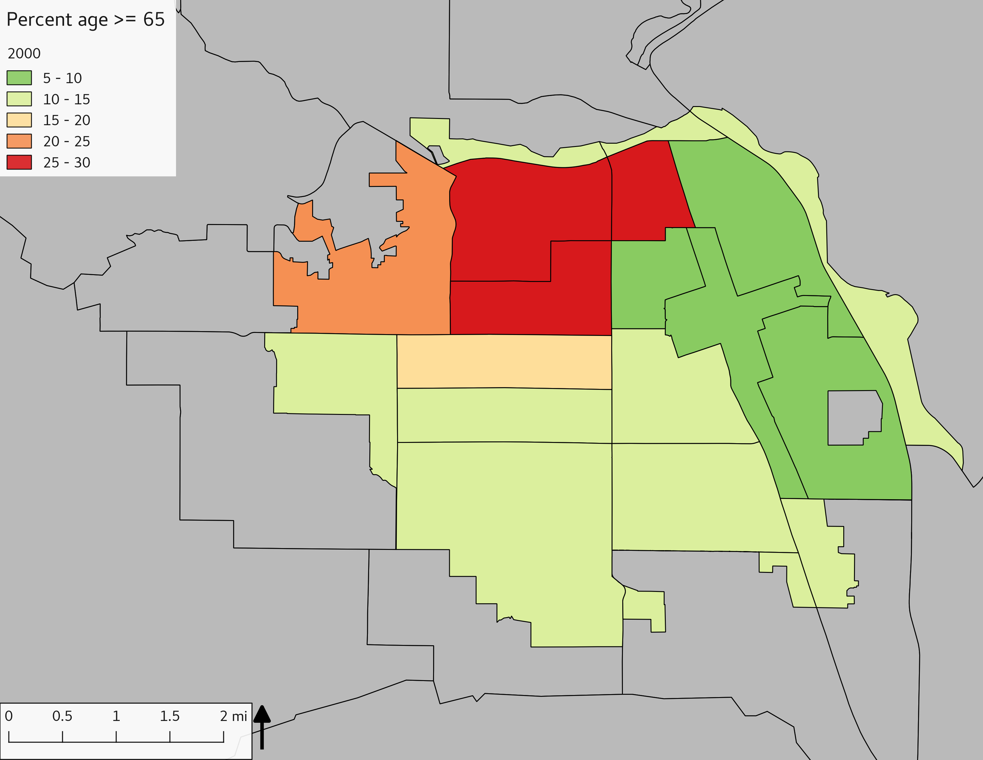
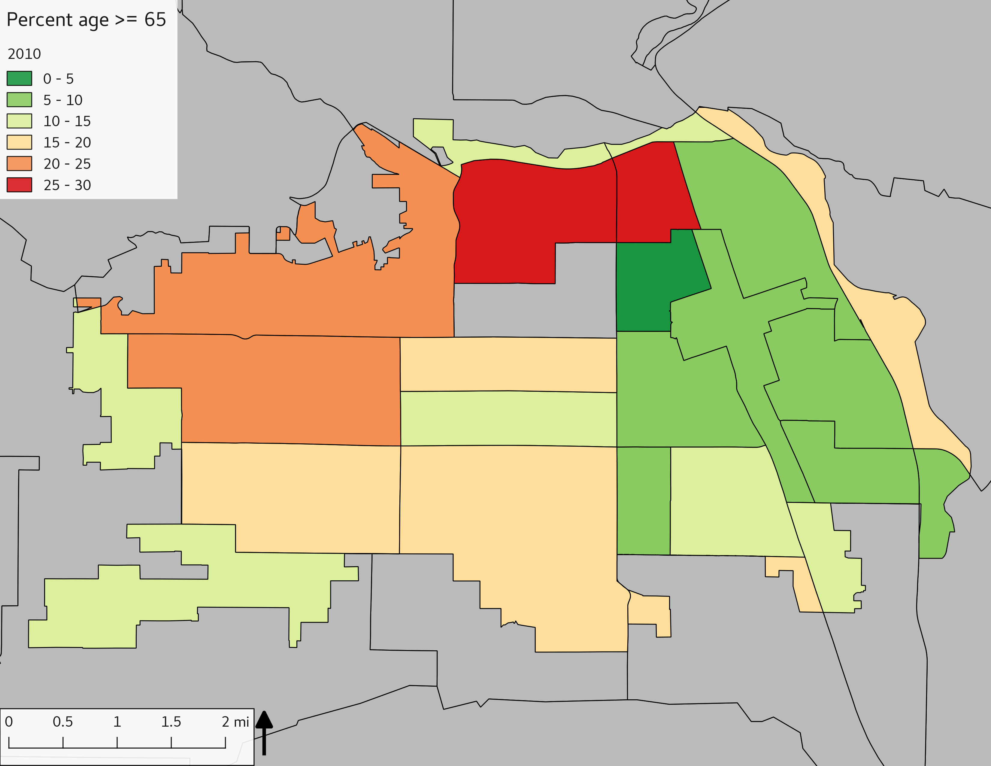
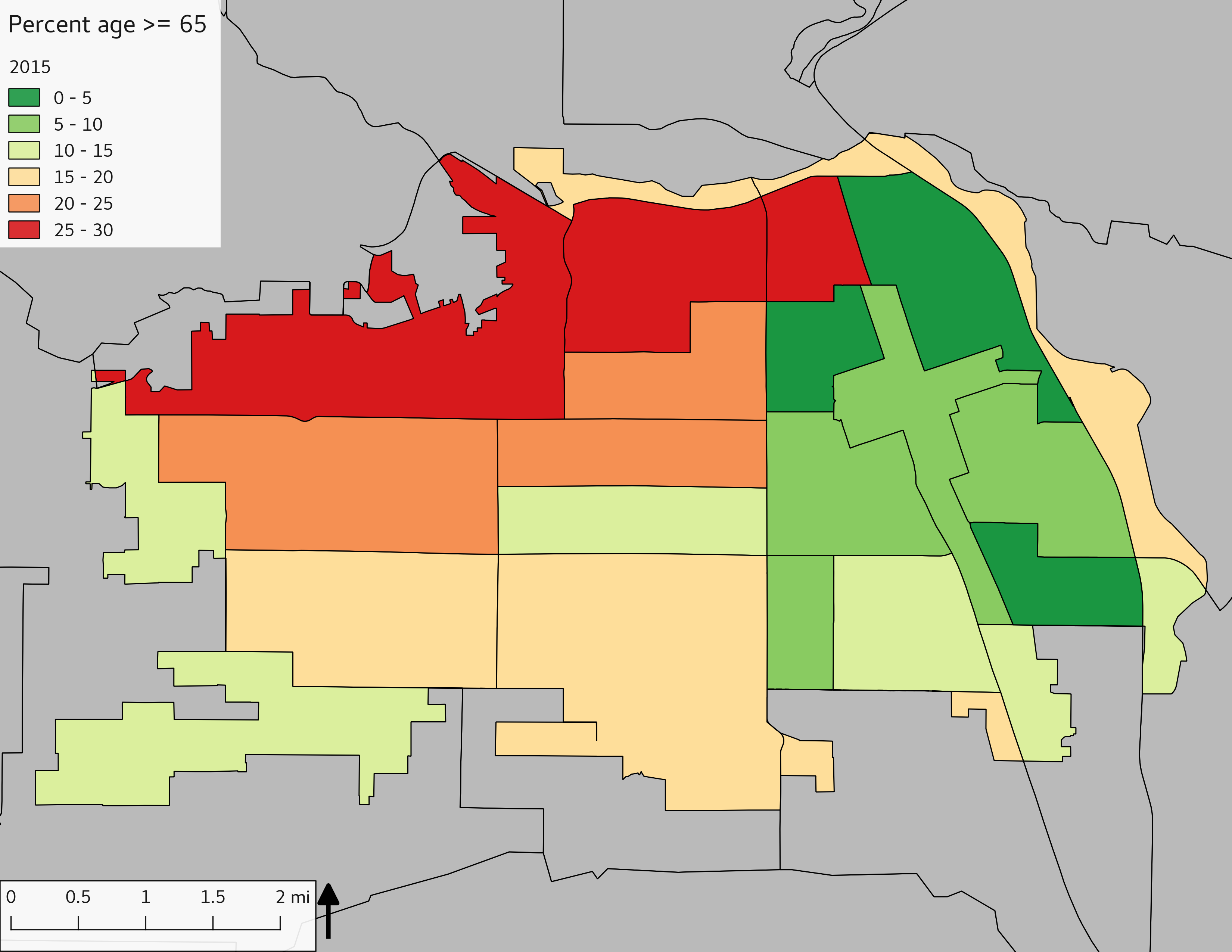
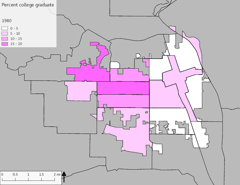
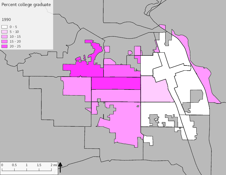
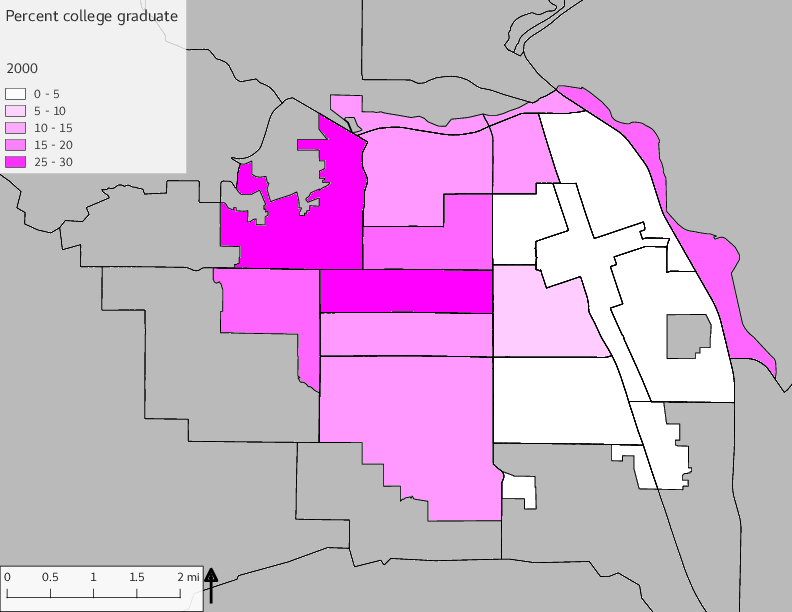
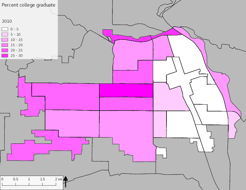
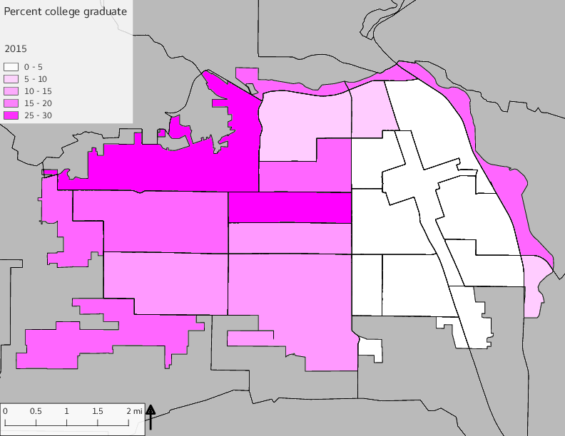
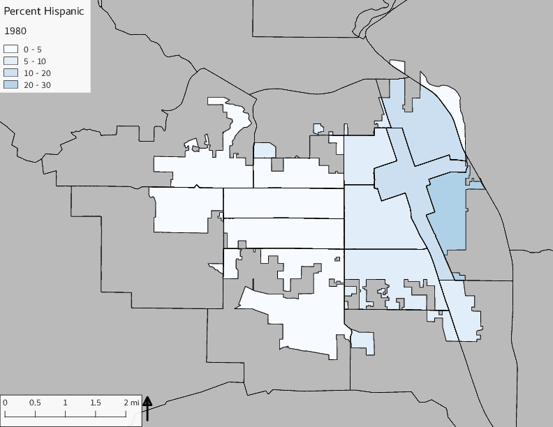
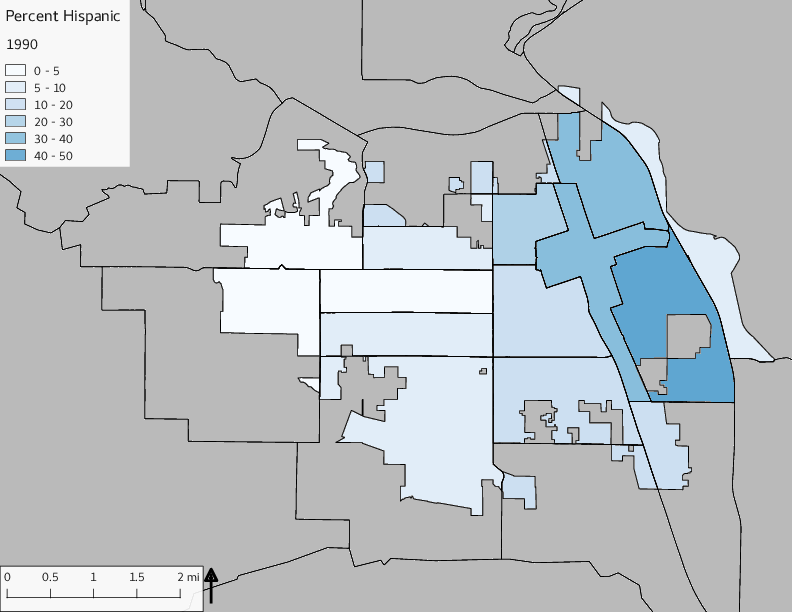
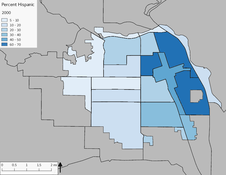
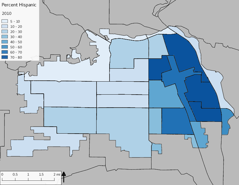
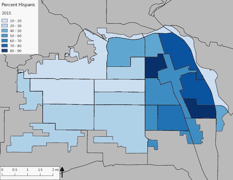
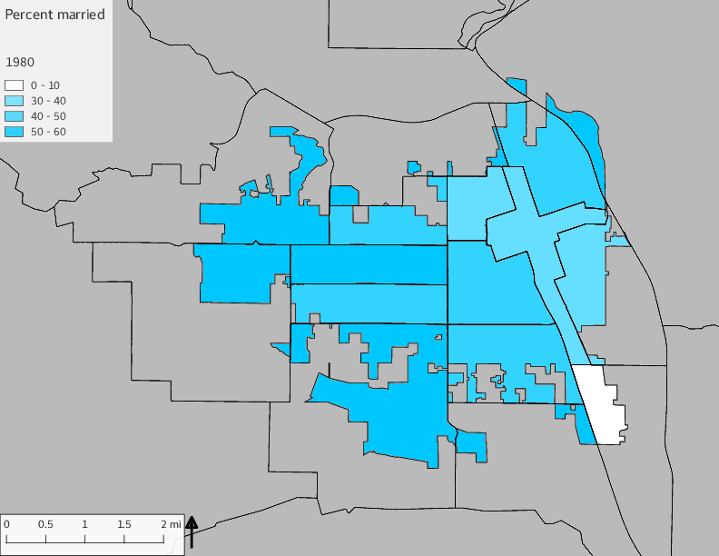
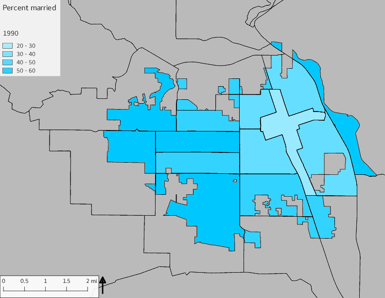
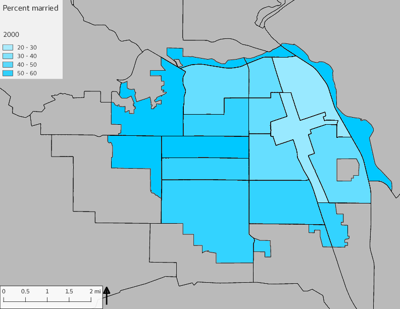
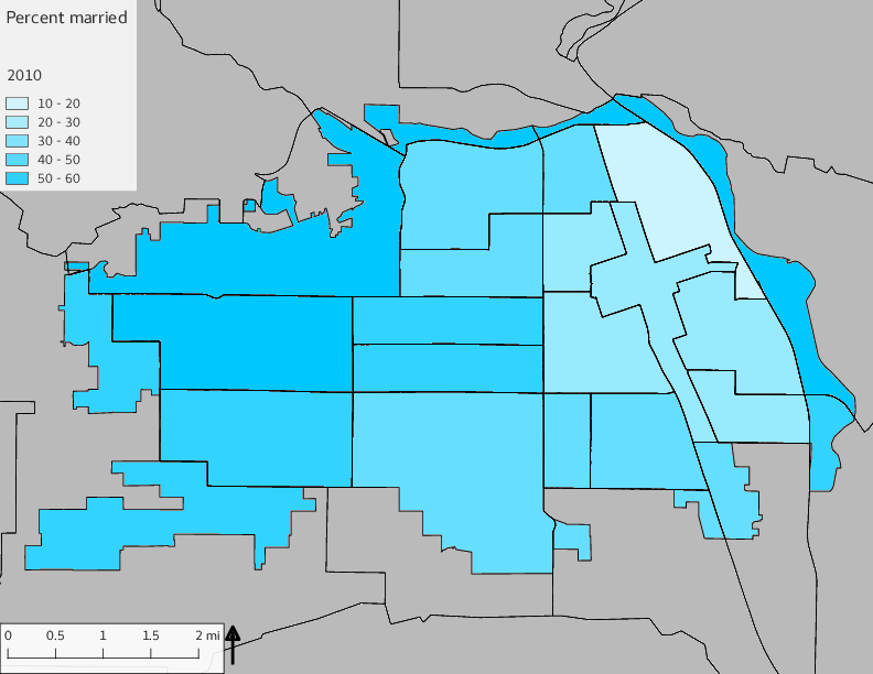
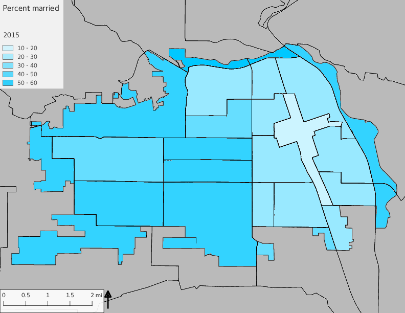
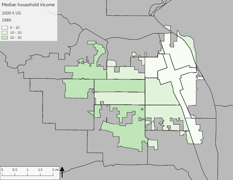
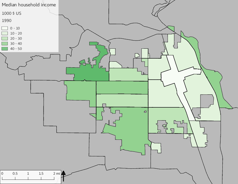
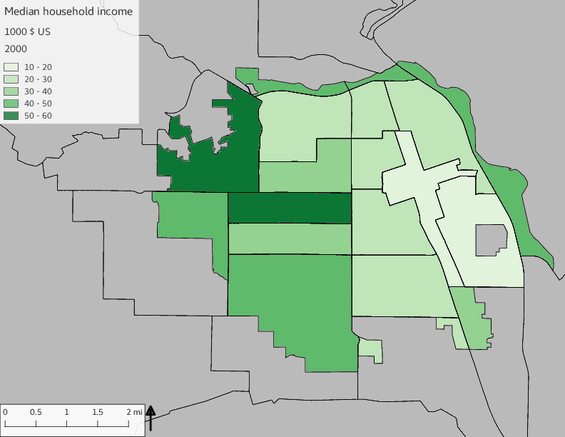
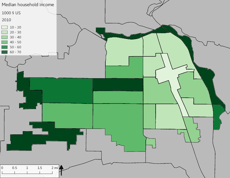
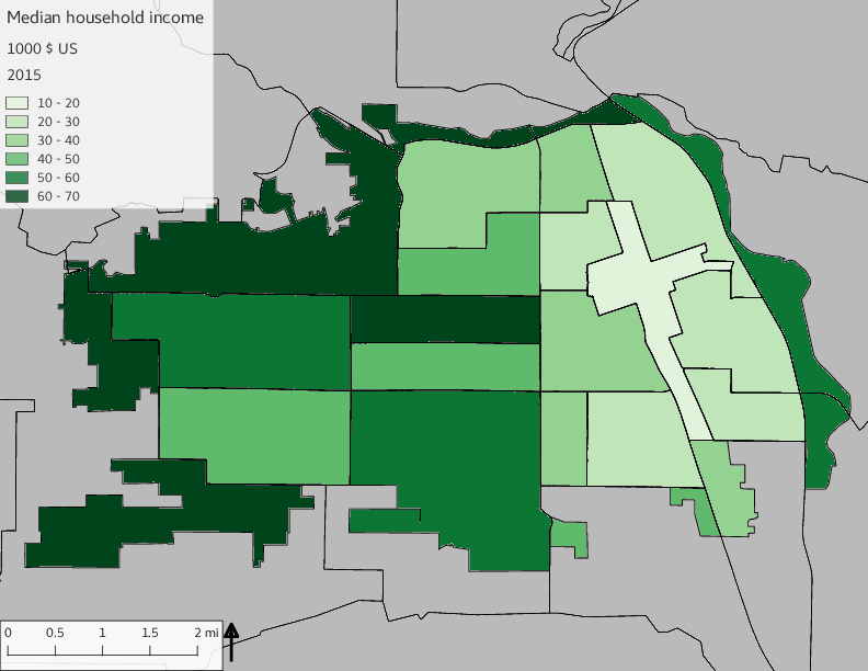
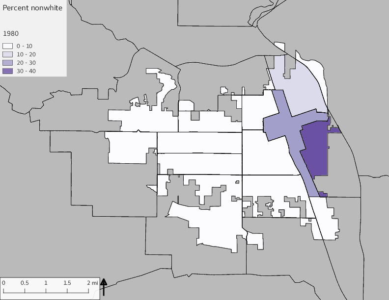
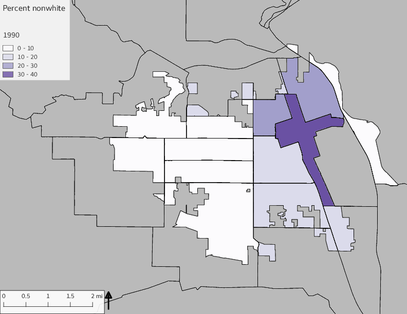
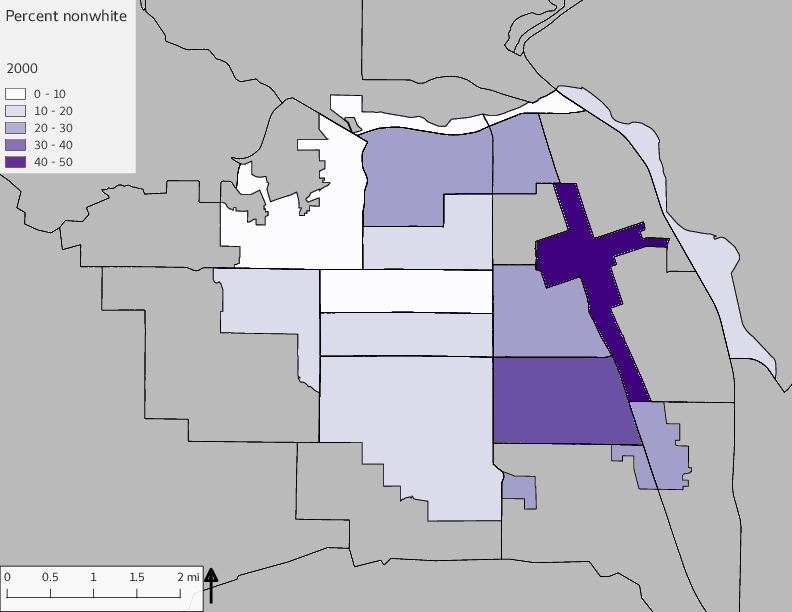
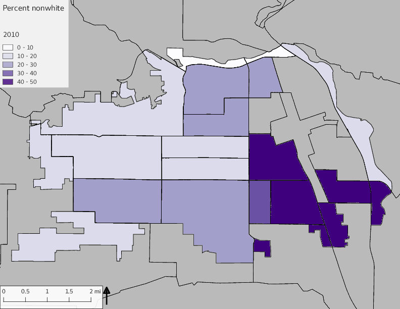
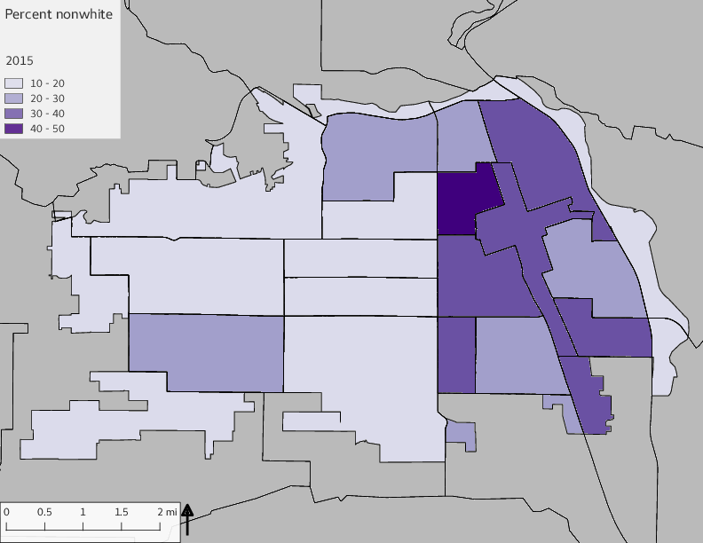
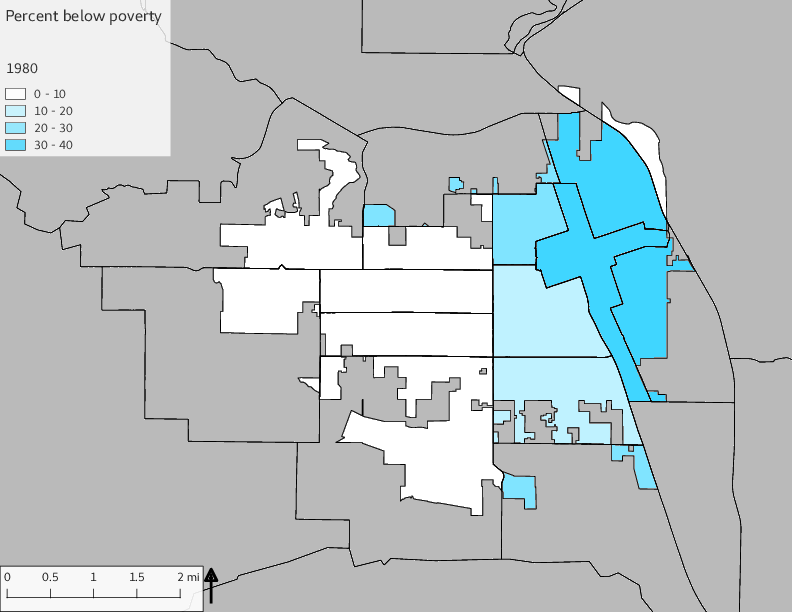
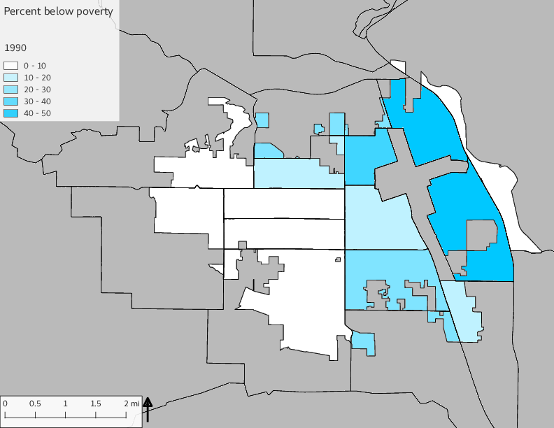
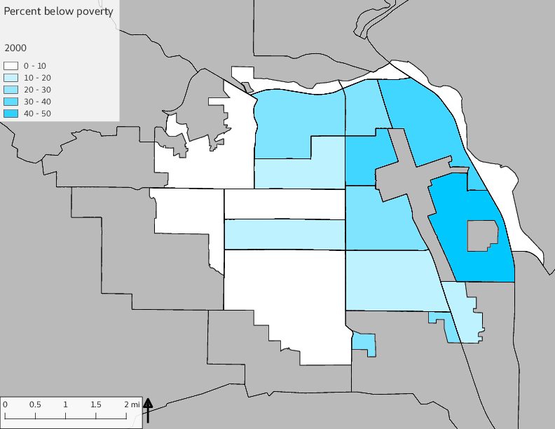
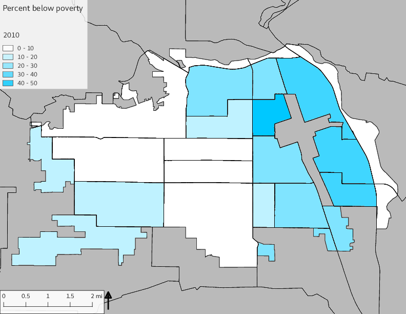
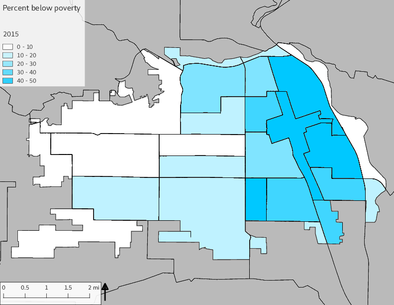
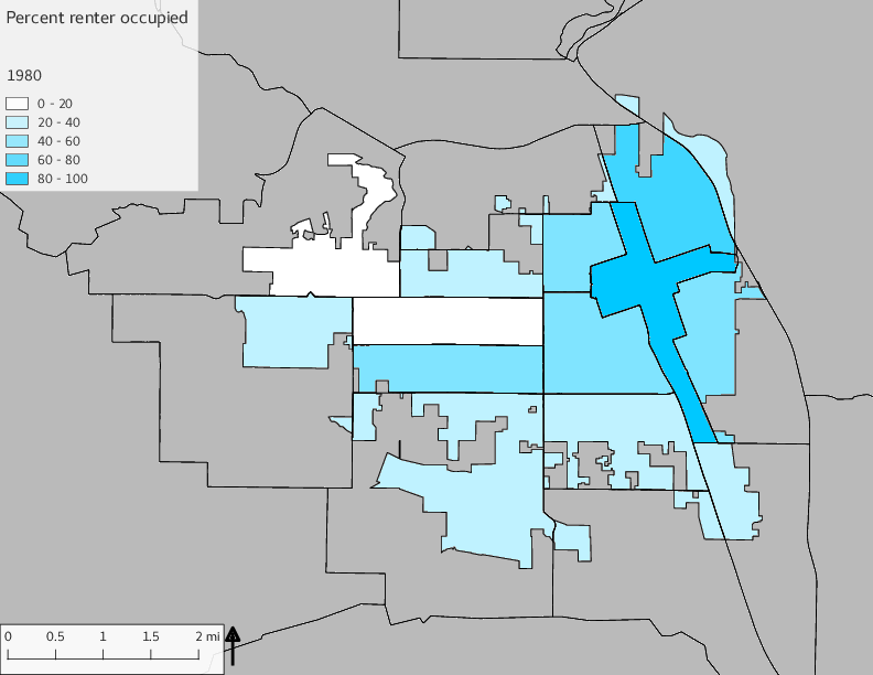
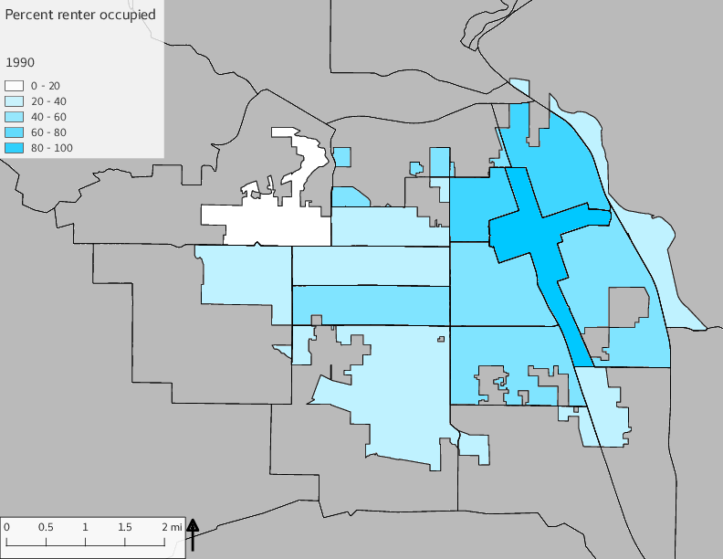
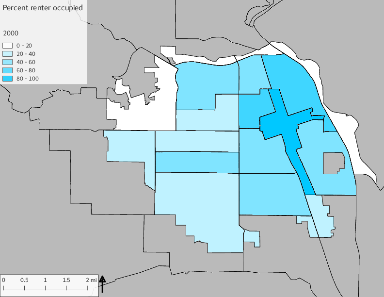
The set of demographic characteristic maps show changes in the values of demographic values over time.
include_graphics(othermaps)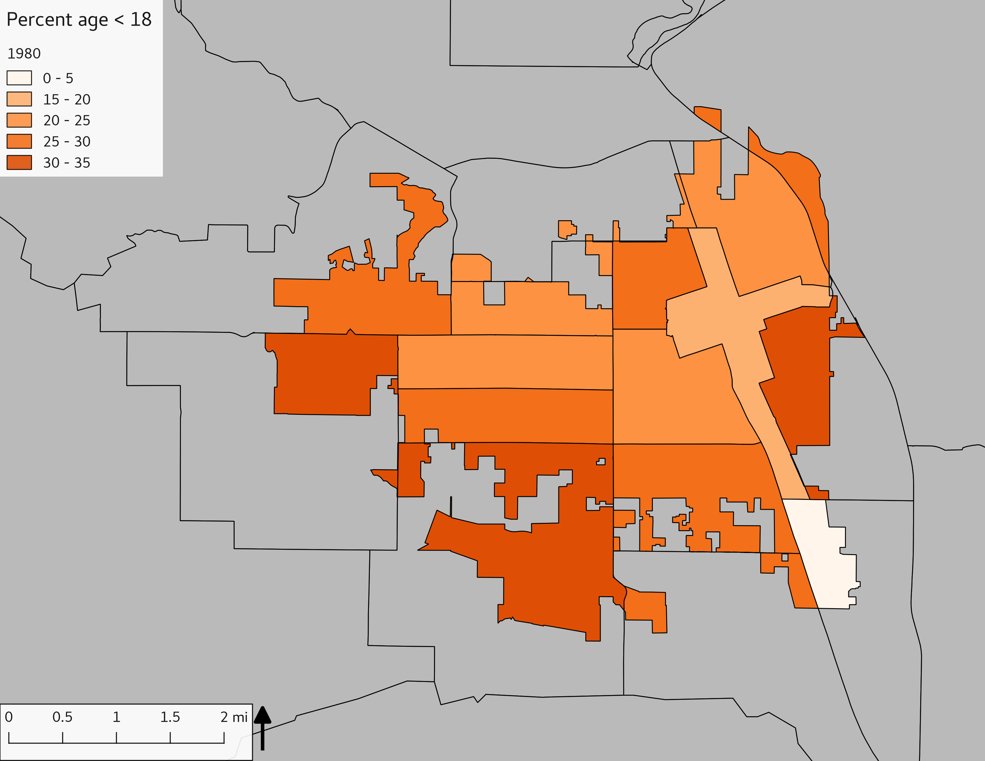
3.3 Historical infrastructure/services allocation
ntracts80 <- dbGetQuery(conn = dbconn, statement = "with a as (select * from yakima_equity.tract_1980)
                                    , b as (select st_union(the_geom_2286) as geom from yakima_equity.annexations where extract('year' from annex_date) <= 1980)
                                    select count(a.*) from a, b where st_intersects(a.the_geom_2286, b.geom);")$count

                                ntractswithpark1980_all <- dbGetQuery(conn = dbconn, statement = "with a as (select * from yakima_equity.tract_1980)
                                    , b as (select st_union(the_geom_2286) as geom from yakima_equity.annexations where extract('year' from annex_date) <= 1980)
                                    , prp as (select * from yakima_equity.park_private)
                                    , p0 as (select * from yakima_equity.parksvalid where yearcreated <= 1980 and yearcreated is not null)
                                    , p as (select name, the_geom_2286, st_area(the_geom_2286) as park_area_orig from p0)
                                    , ai as (select a.* from a, b where st_intersects(a.the_geom_2286, b.geom))
                                    , f as (select * from ai, p where st_intersects(ai.the_geom_2286, p.the_geom_2286))
                                    select count(distinct tract) from f;")$count

                                ntractswithpark1980 <- dbGetQuery(conn = dbconn, statement = "with a as (select * from yakima_equity.tract_1980)
                                    , b as (select st_union(the_geom_2286) as geom from yakima_equity.annexations where extract('year' from annex_date) <= 1980)
                                    , prp as (select * from yakima_equity.park_private)
                                    , p0 as (select * from yakima_equity.parksvalid where yearcreated <= 1980 and yearcreated is not null and name not in (select name from prp))
                                    , p as (select name, the_geom_2286, st_area(the_geom_2286) as park_area_orig from p0)
                                    , ai as (select a.* from a, b where st_intersects(a.the_geom_2286, b.geom))
                                    , f as (select * from ai, p where st_intersects(ai.the_geom_2286, p.the_geom_2286))
                                    select count(distinct tract) from f;")$count

                                ntracts2015 <- dbGetQuery(conn = dbconn, statement = "with a as (select * from yakima_equity.tract_2015)
                                    , b as (select st_union(the_geom_2286) as geom from yakima_equity.annexations where extract('year' from annex_date) <= 2015)
                                    select count(a.*) from a, b where st_intersects(a.the_geom_2286, b.geom);")$count

                                ntractswithpark2015_all <- dbGetQuery(conn = dbconn, statement = "with a as (select * from yakima_equity.tract_2015)
                                    , b as (select st_union(the_geom_2286) as geom from yakima_equity.annexations where extract('year' from annex_date) <= 2015)
                                    , prp as (select * from yakima_equity.park_private)
                                    , p0 as (select * from yakima_equity.parksvalid where yearcreated <= 1980 and yearcreated is not null)
                                    , p as (select name, the_geom_2286, st_area(the_geom_2286) as park_area_orig from p0)
                                    , ai as (select a.* from a, b where st_intersects(a.the_geom_2286, b.geom))
                                    , f as (select * from ai, p where st_intersects(ai.the_geom_2286, p.the_geom_2286))
                                    select count(distinct tract) from f;")$count

                                ntractswithpark2015 <- dbGetQuery(conn = dbconn, statement = "with a as (select * from yakima_equity.tract_2015)
                                    , b as (select st_union(the_geom_2286) as geom from yakima_equity.annexations where extract('year' from annex_date) <= 2015)
                                    , prp as (select * from yakima_equity.park_private)
                                    , p0 as (select * from yakima_equity.parksvalid where yearcreated <= 1980 and yearcreated is not null and name not in (select name from prp))
                                    , p as (select name, the_geom_2286, st_area(the_geom_2286) as park_area_orig from p0)
                                    , ai as (select a.* from a, b where st_intersects(a.the_geom_2286, b.geom))
                                    , f as (select * from ai, p where st_intersects(ai.the_geom_2286, p.the_geom_2286))
                                    select count(distinct tract) from f;")$count
A set of graphs is shown below; each graph displays the data point along with the tract numeric identifier.
These graphs should be interpreted with caution due to implicit assumptions/limitations:
- The data shown were analyzed using census tracts. Use of census tracts for area-weighted summary assumes that the census population estimates are correct, and that populations are uniformly distributed and uniformly heterogeneous across the tract. It also assumes that all persons residing within the tract have equal access to the parks within the tract, and that persons residing in one tract have access to only those parks within that tract.
- The data are quite sparse; there were only 17 census tracts in 1980 and 24 tracts in 2015; only 10 of those in 1980 (and 12 in 2015) had parks overlapping the tract boundary. Because of the small sample sizes, no formal statistical tests were possible. Also, because of the small sample sizes, “outlier” points could have a strong leverage effect on any observed trends, so regression trend lines were not added to the graphs.
3.3.1 Parks
Parks are shown in the map:
include_graphics(parkmaps)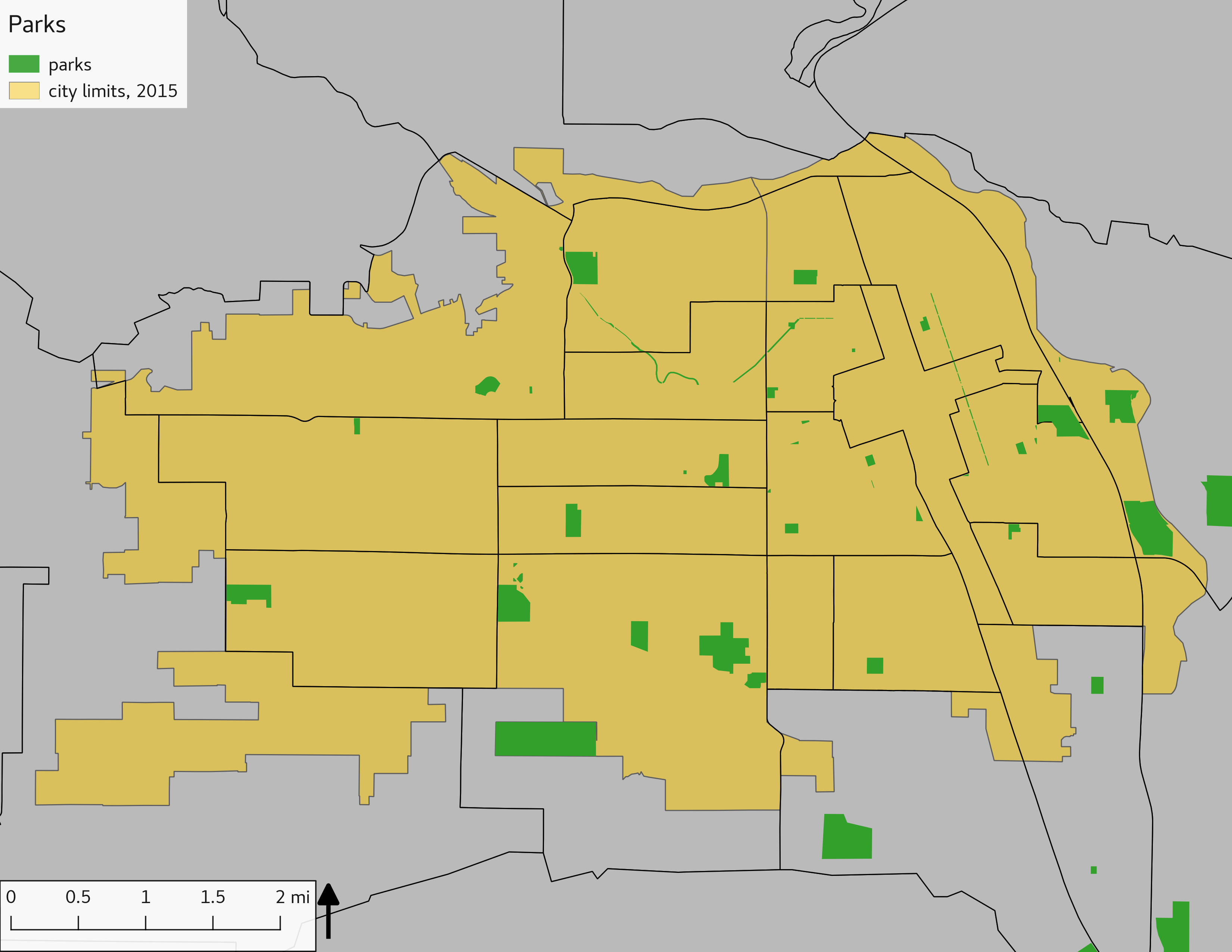
3.3.1.1 Area of parks in Yakima stratified by 16th Avenue
The graph shows the area of park per capita of tract across years and stratified by the 16th Avenue dividing line. There is more area in parks per capita west of 16th Avenue than east, a trend that continued over time; however, the relative difference lessened over time.
sql <- "
                                        with
                                        --parks
                                        p0 as (select * from yakima_equity.parksvalid where yearcreated <= xxxYEARxxx)
                                        , p as (select row_number() over() as pid, the_geom_2286 from p0)
                                        --annexation as single poly
                                        , anx as (select st_union(the_geom_2286) as geom from yakima_equity.annexations where extract('year' from annex_date) <= xxxYEARxxx)
                                        --census tracts
                                        , ct as (select tract, zone_16th, st_area(the_geom_2286) as area_ct, total_pop, the_geom_2286 from yakima_equity.tract_xxxYEARxxx)
                                        --sum population e/w
                                        , popew_sum as (select zone_16th, sum(total_pop) as pop from ct group by zone_16th)
                                        --parks east west
                                        , pew as (select zone_16th, pid, st_area(st_intersection(p.the_geom_2286, ct.the_geom_2286)) as area_park from p, ct where st_intersects(p.the_geom_2286, ct.the_geom_2286))
                                        --sum park area e/w
                                        , pew_sum as (select zone_16th, sum(area_park) as area_park from pew group by zone_16th)
                                        select 'xxxYEARxxx'::text as year, *, area_park / pop as area_park_per_capita from pew_sum join popew_sum using(zone_16th)
                                        ;"

                                        parkew <- NULL
                                        for(y in c(1980, 1990, 2000, 2010, 2015)){
                                            sqly <- gsub("xxxYEARxxx", y, sql)
                                            parkew <- rbind(parkew, dbGetQuery(conn = dbconn, statement = sqly))
                                        }

                                        # plot
                                        g <- ggplot(data = parkew, aes(x = year, y = area_park_per_capita, fill = zone_16th)) +
                                            geom_bar(position = "dodge", stat = "identity") +
                                            labs(y = "area (ft)", title = "Area of parks per capita stratified by 16th Avenue", fill = "16th Ave divide") +
                                            theme(plot.title = element_text(size=12))

                                        print(g)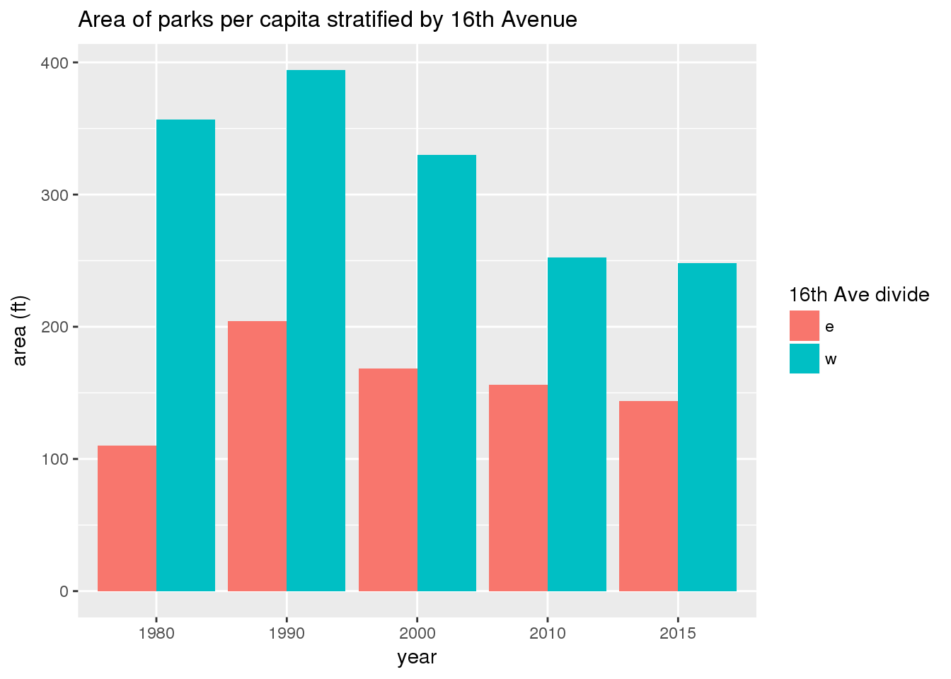
ggsave(filename = file.path(imagedir, "parkarea_16th.png"), plot = g, width = ggsavewidth, height = ggsaveheight, units = "in")3.3.1.2 Park per capita area by census tract demographics
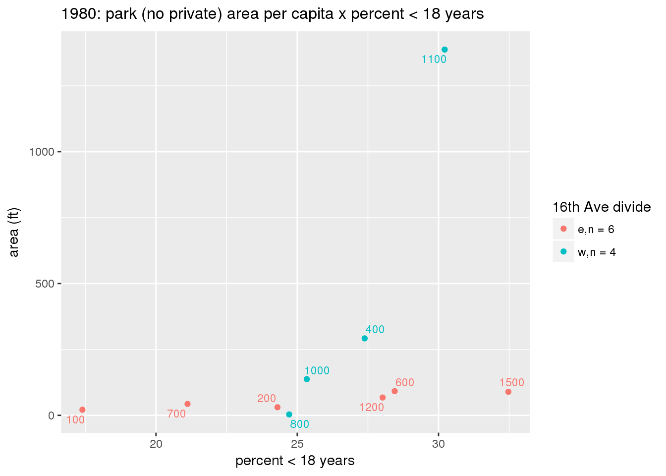
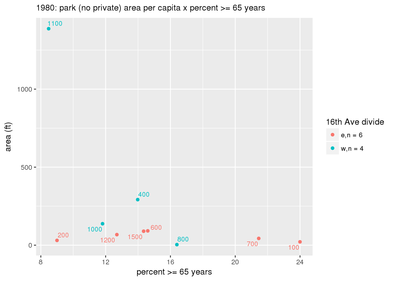
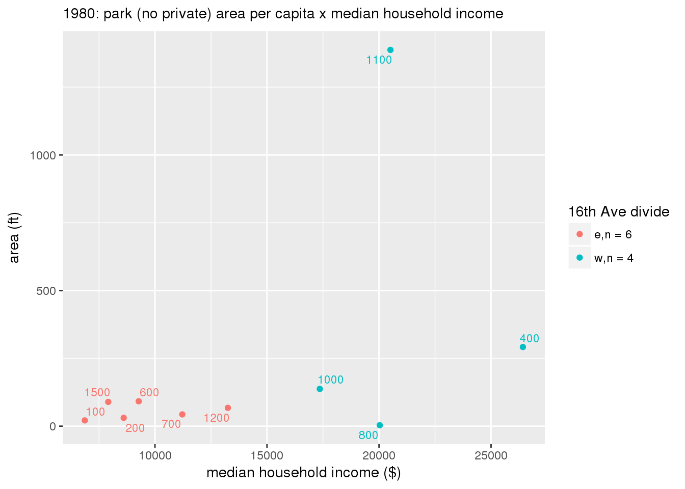
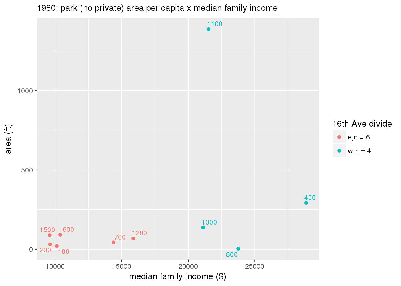
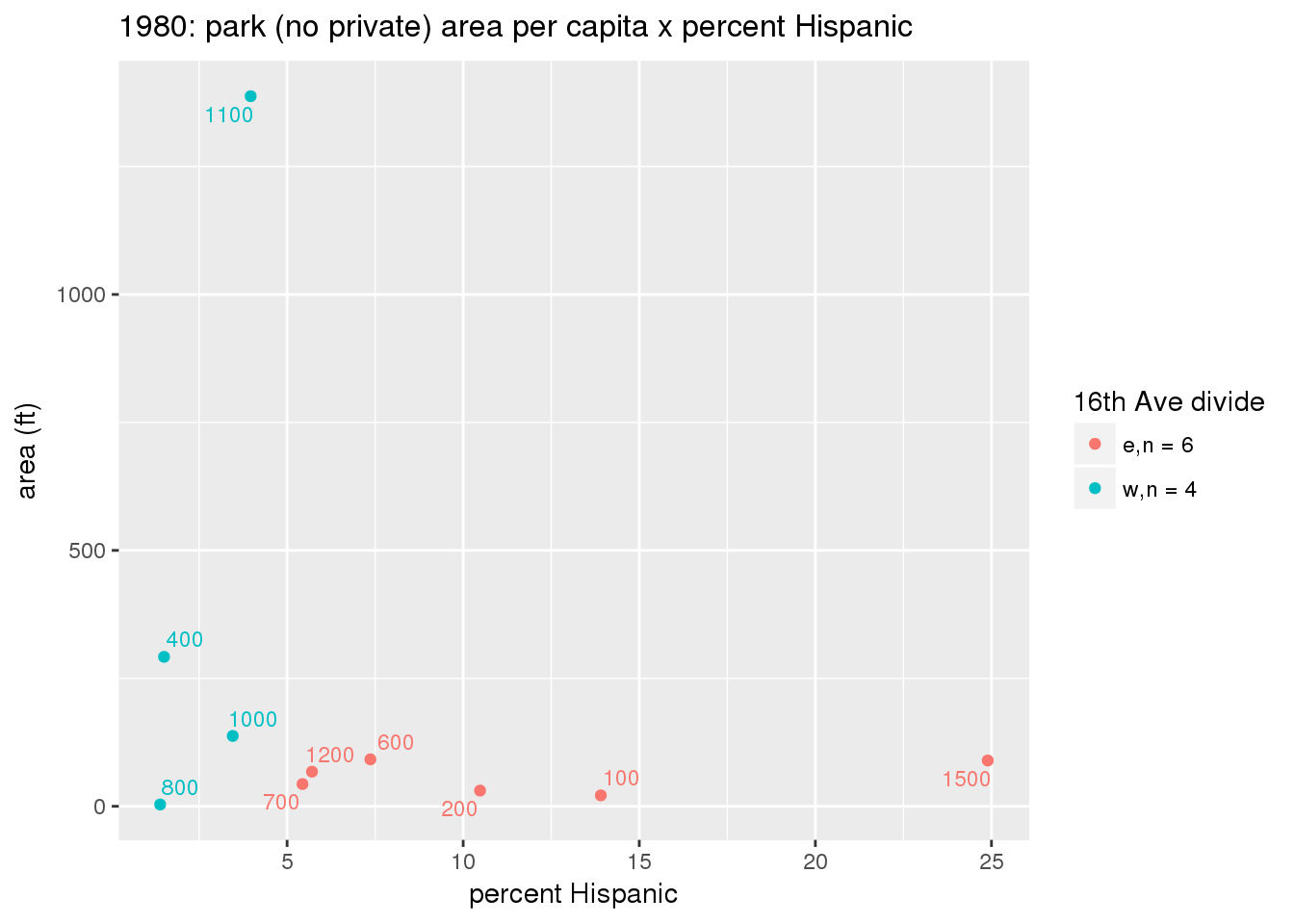
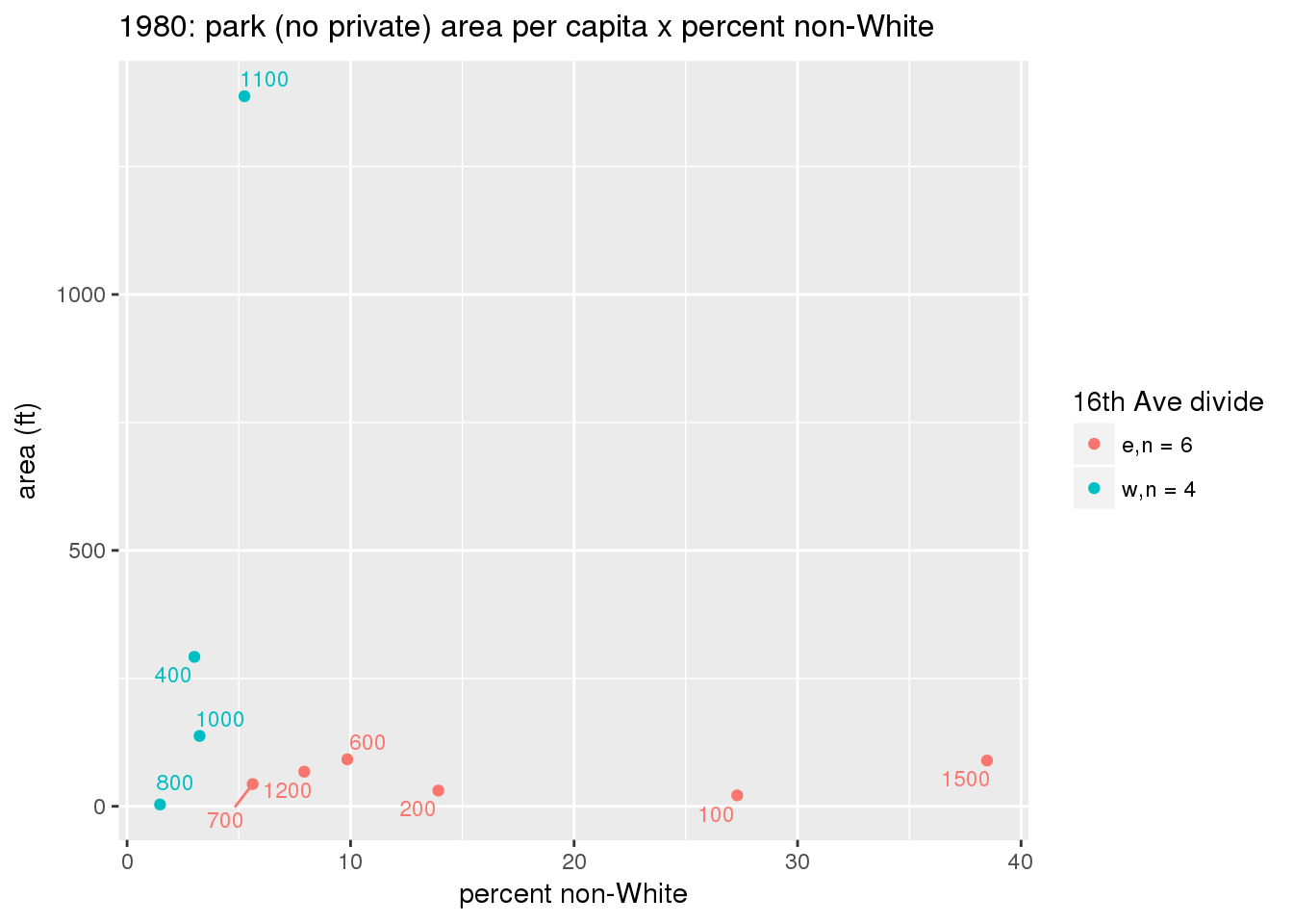
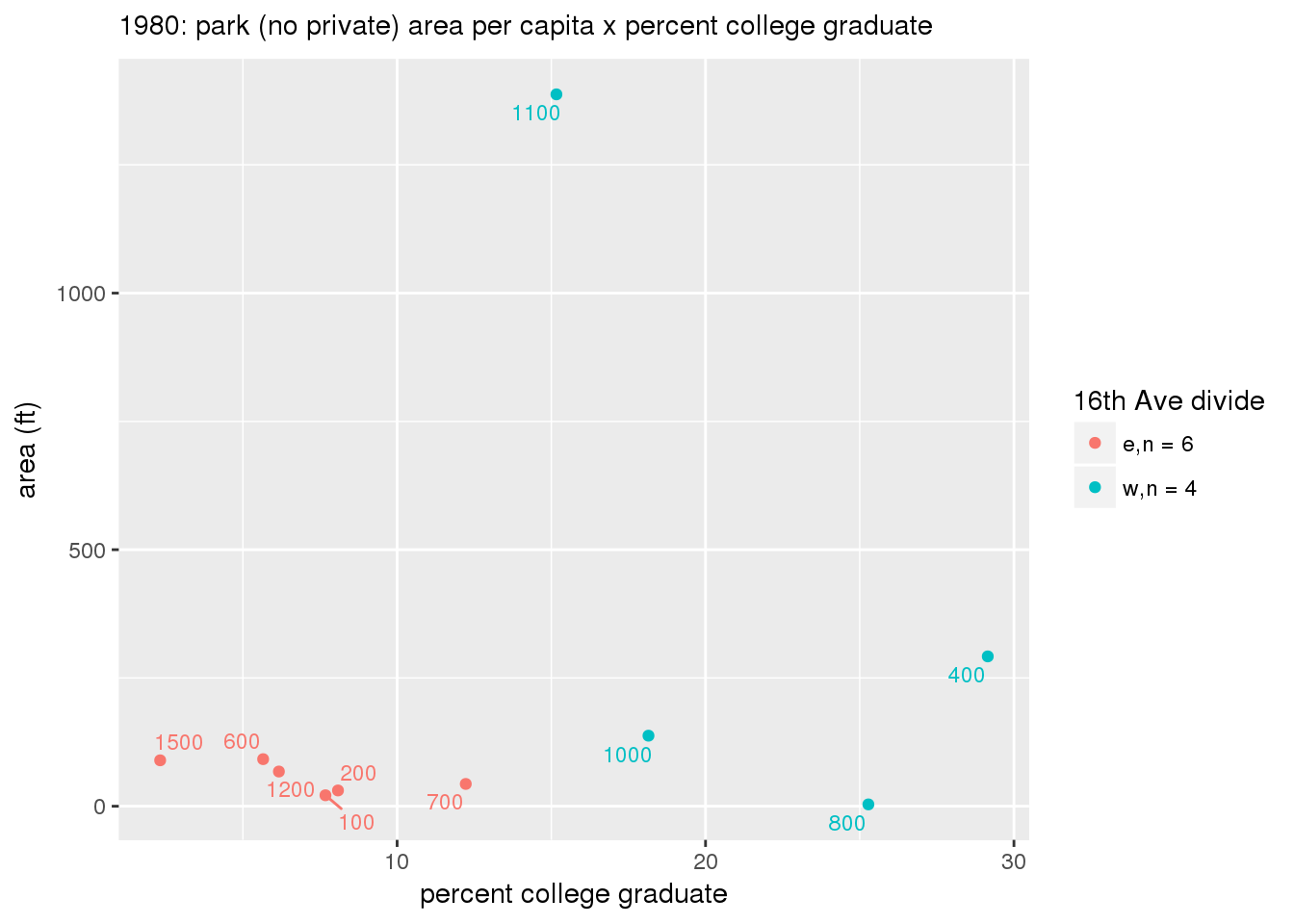
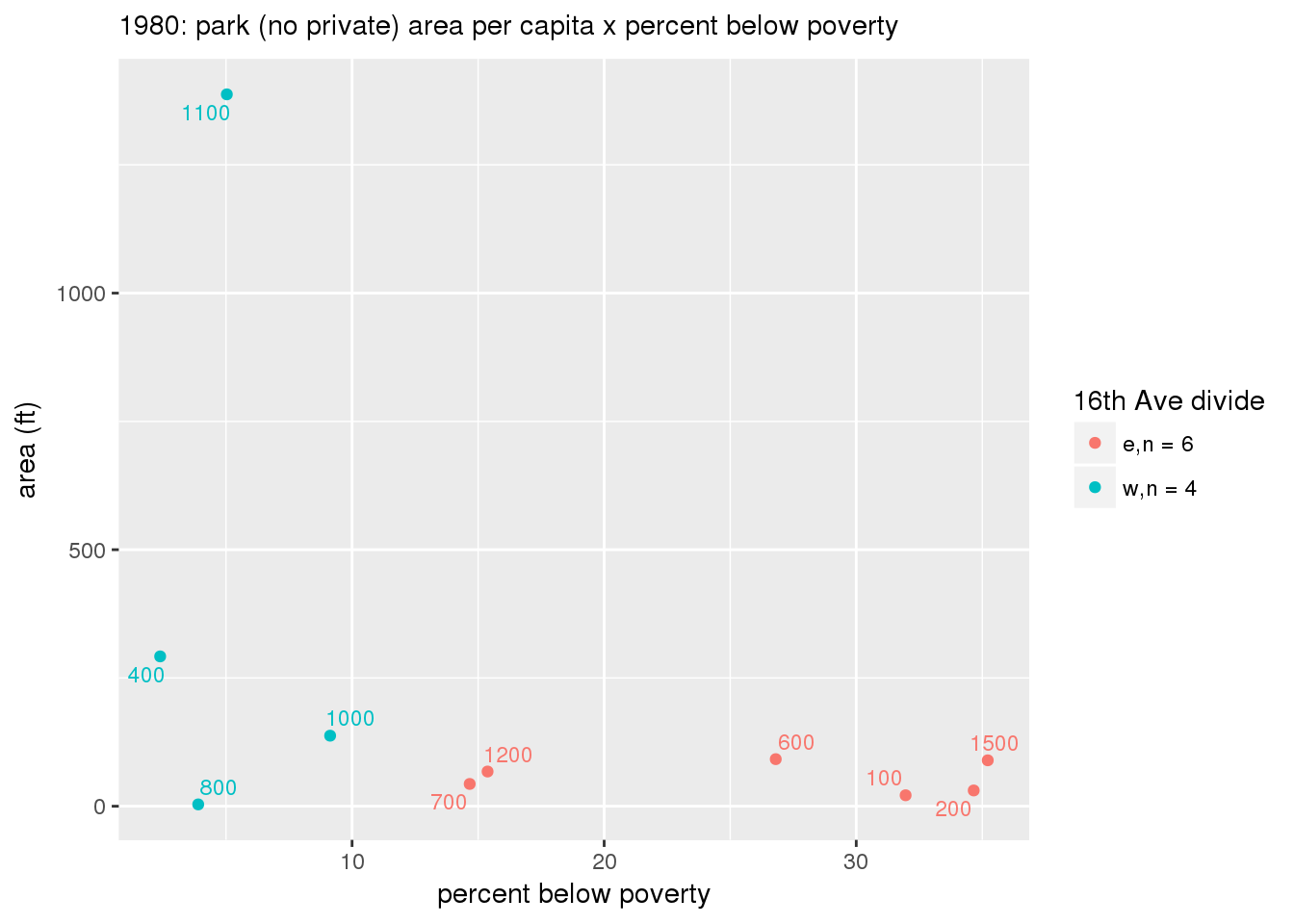
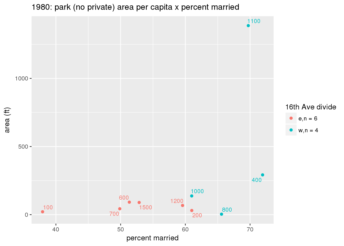
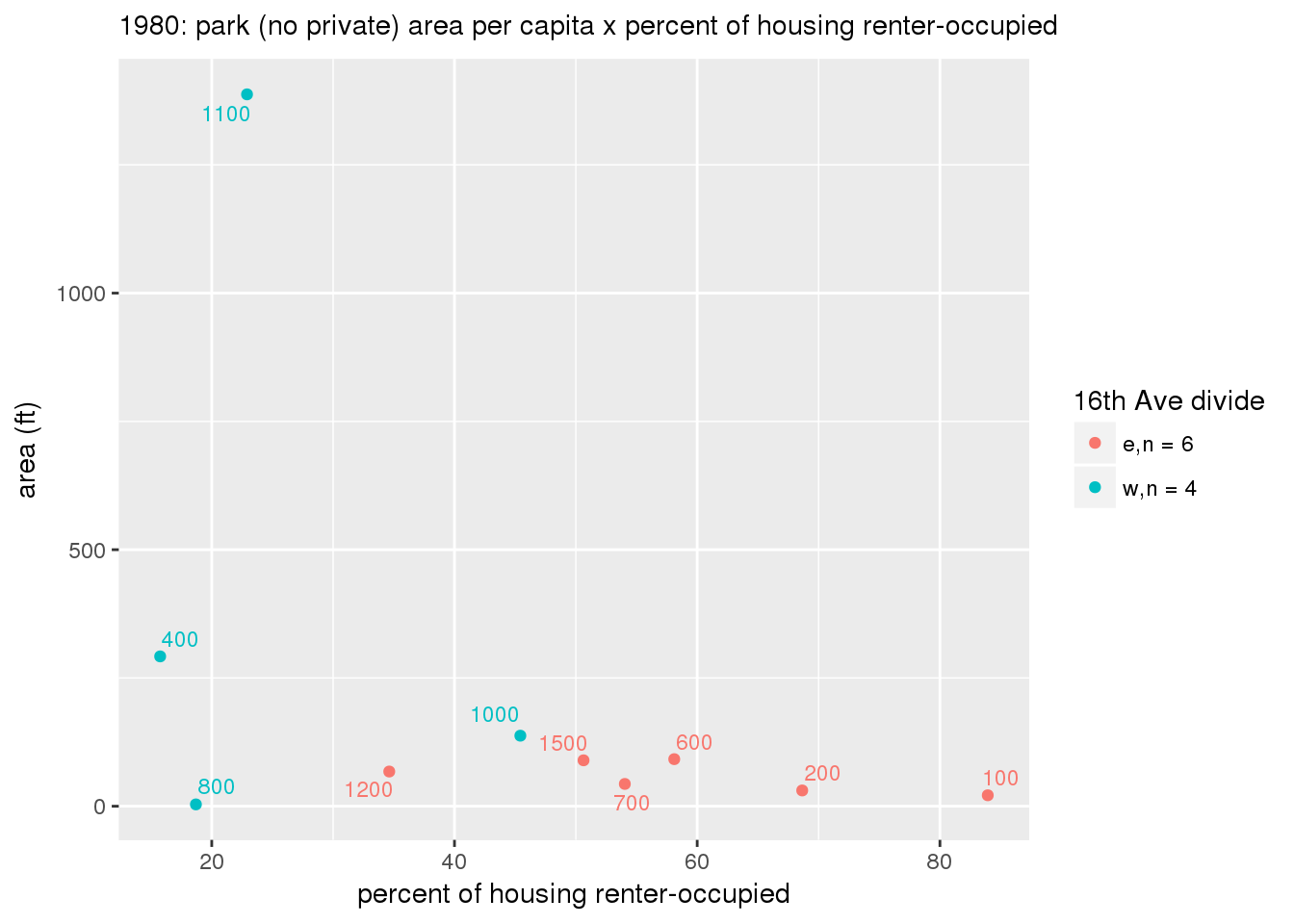
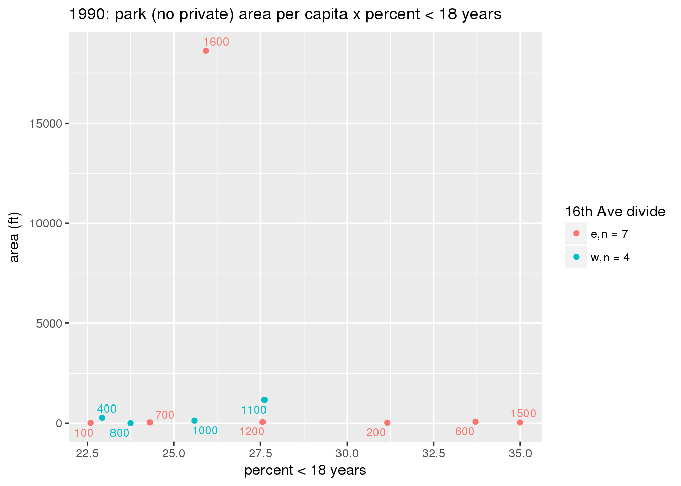
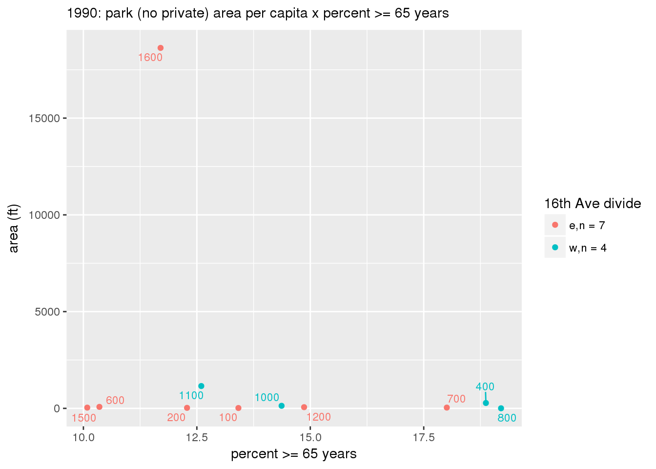
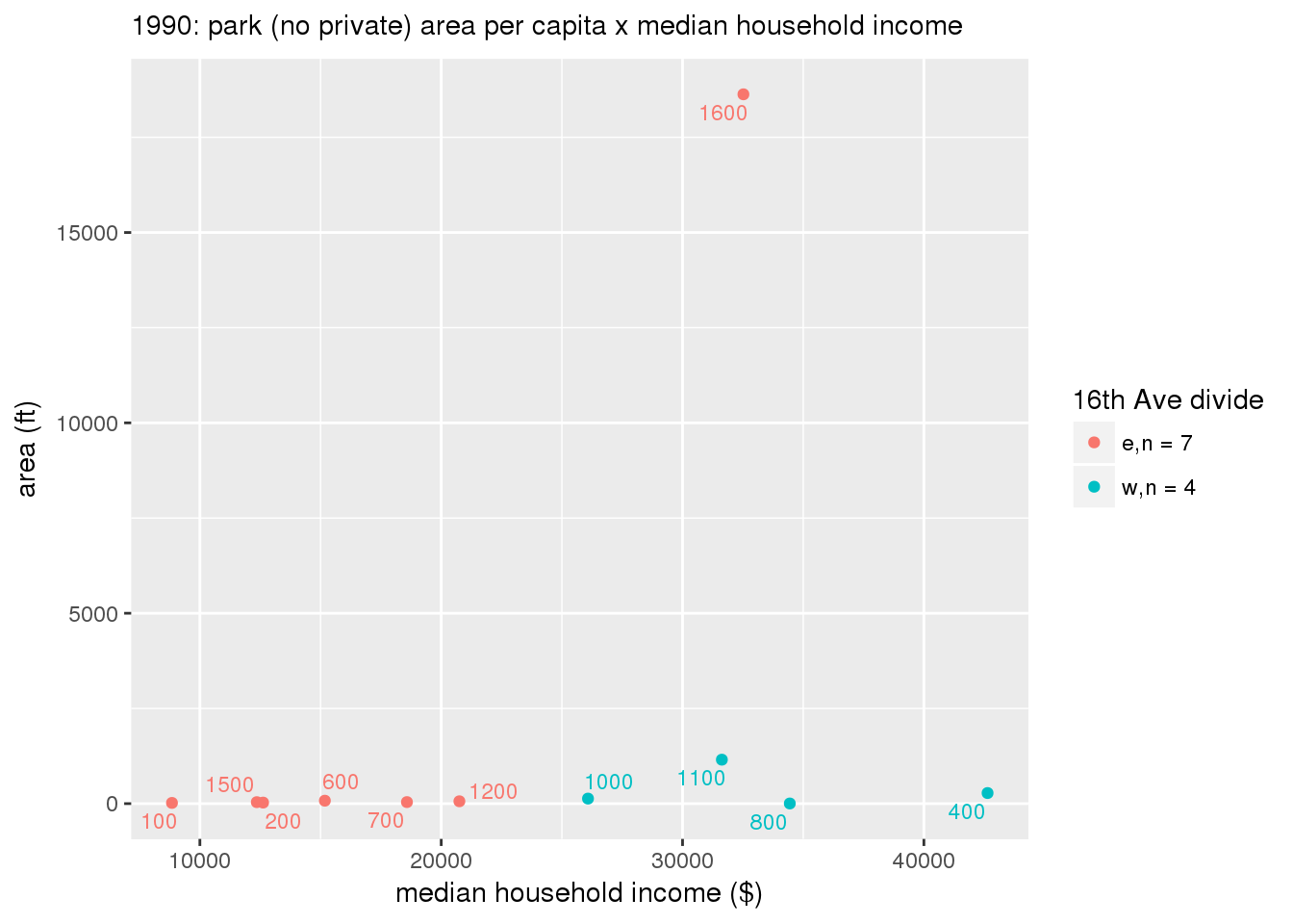
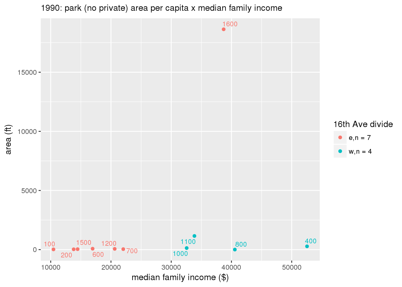
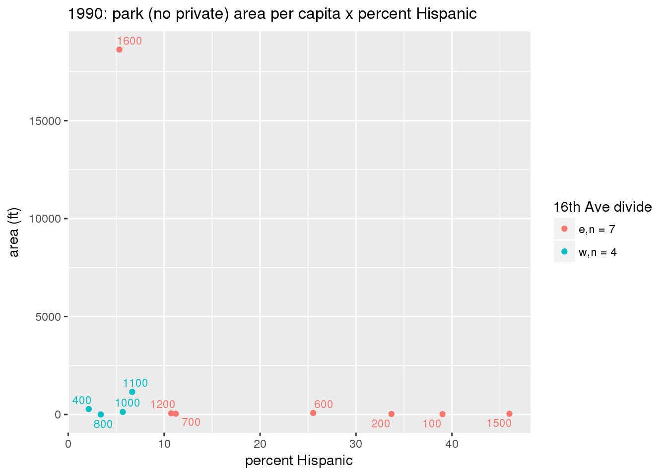
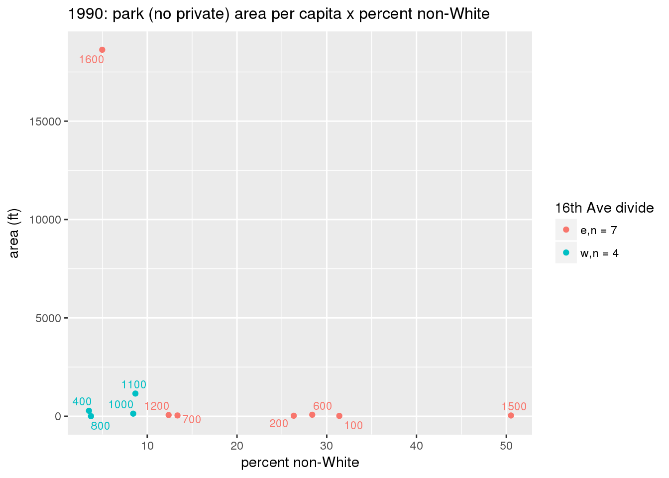
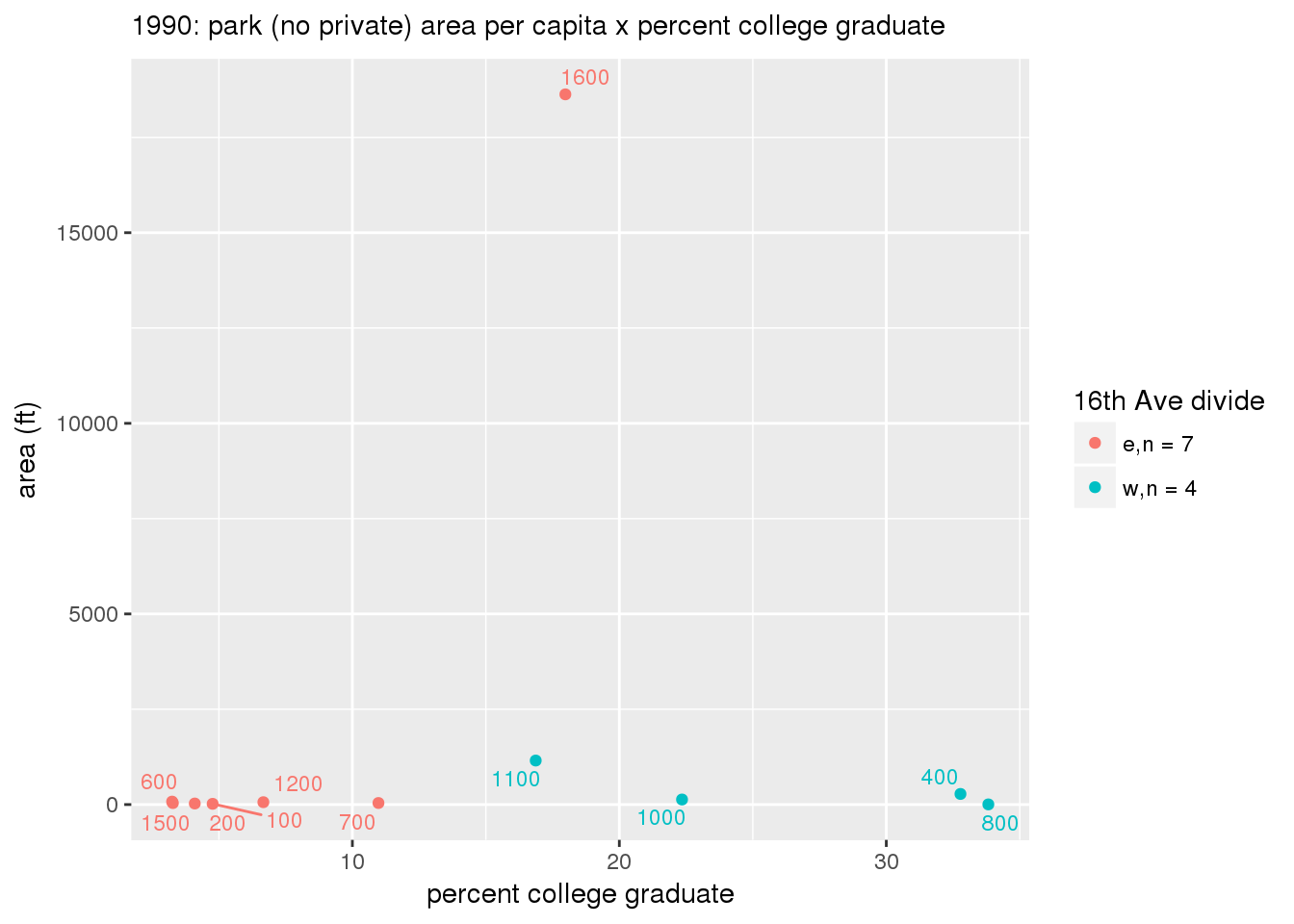
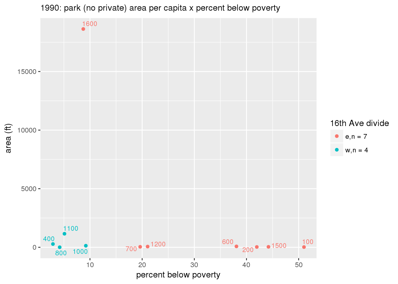
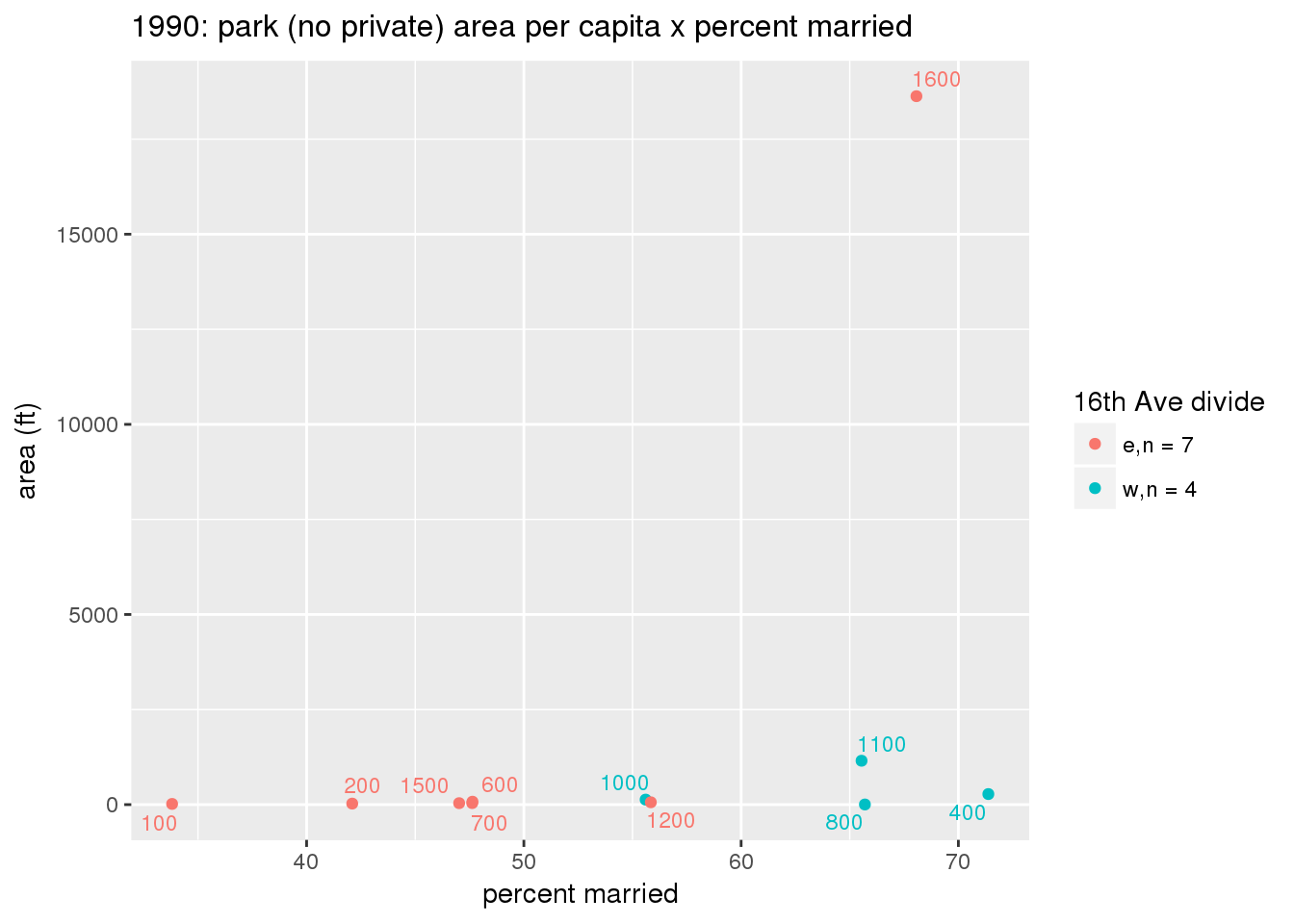
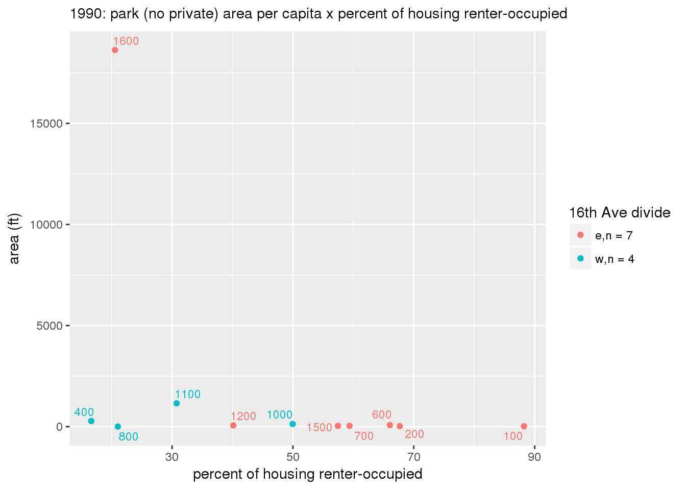
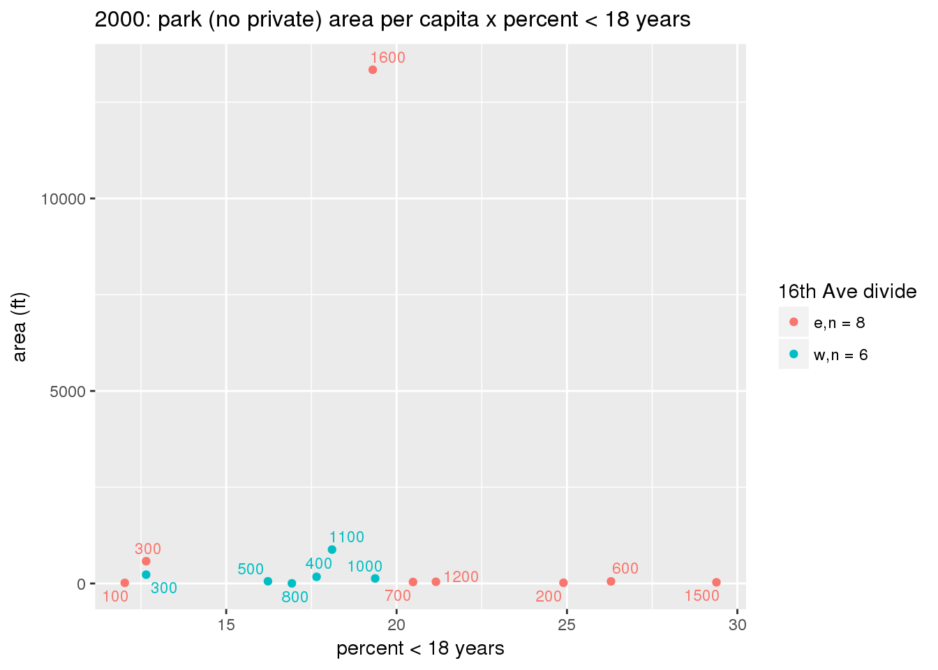
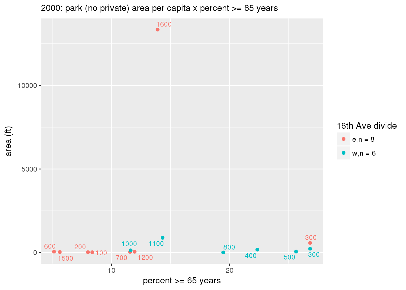
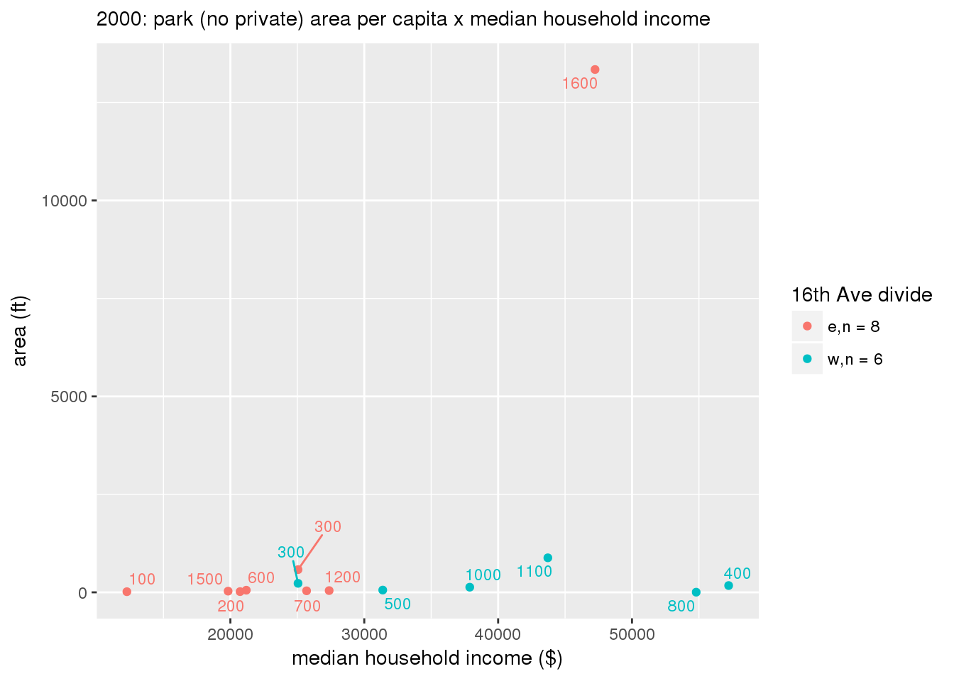
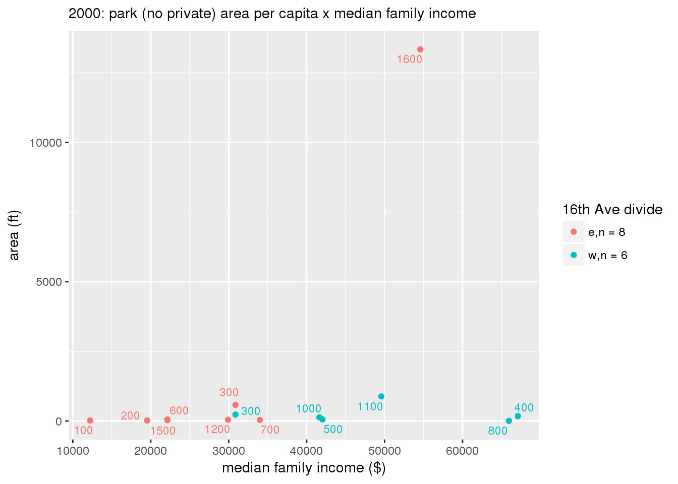
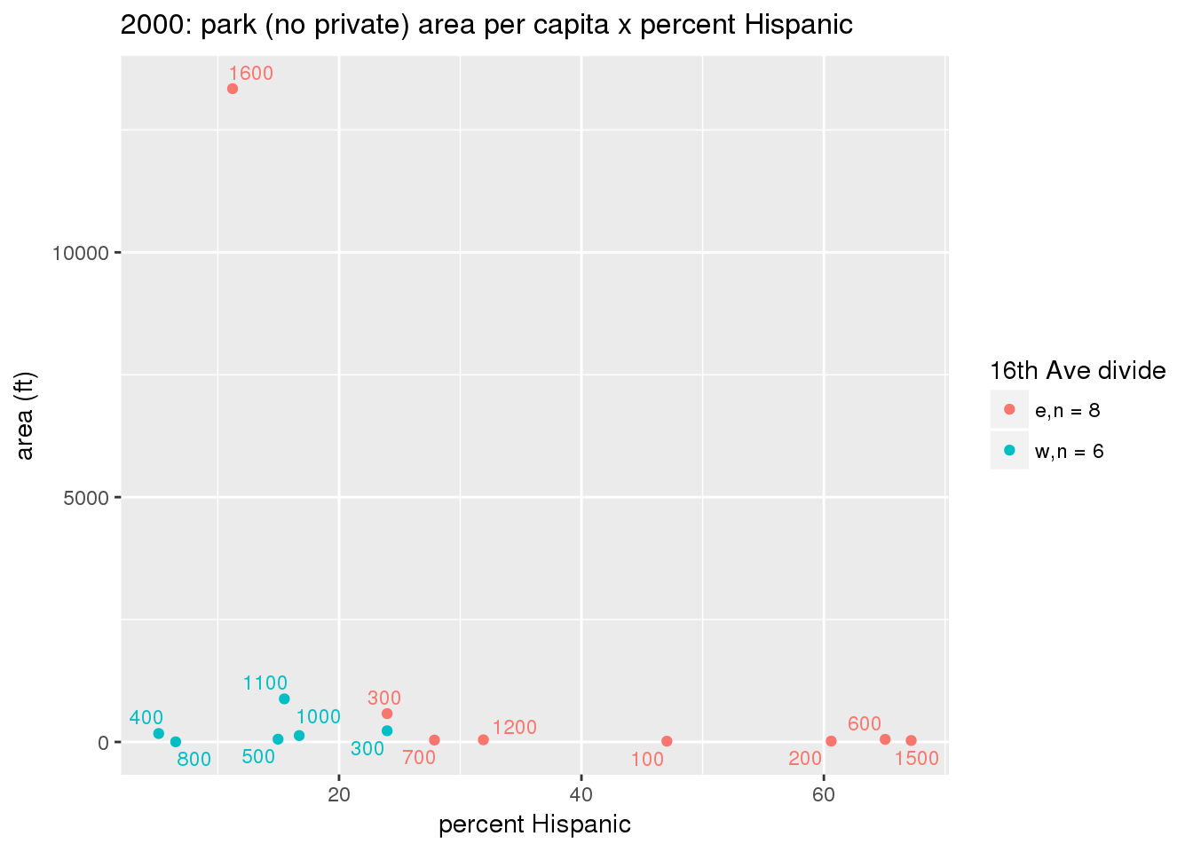
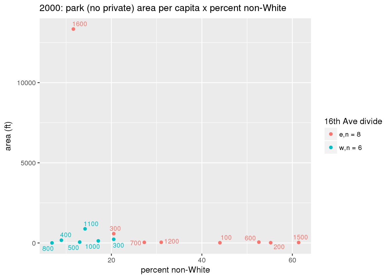
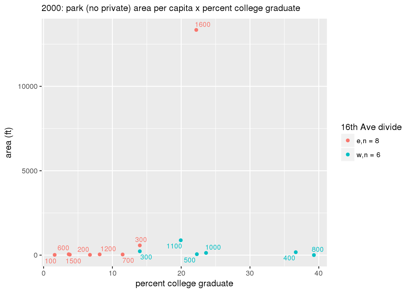
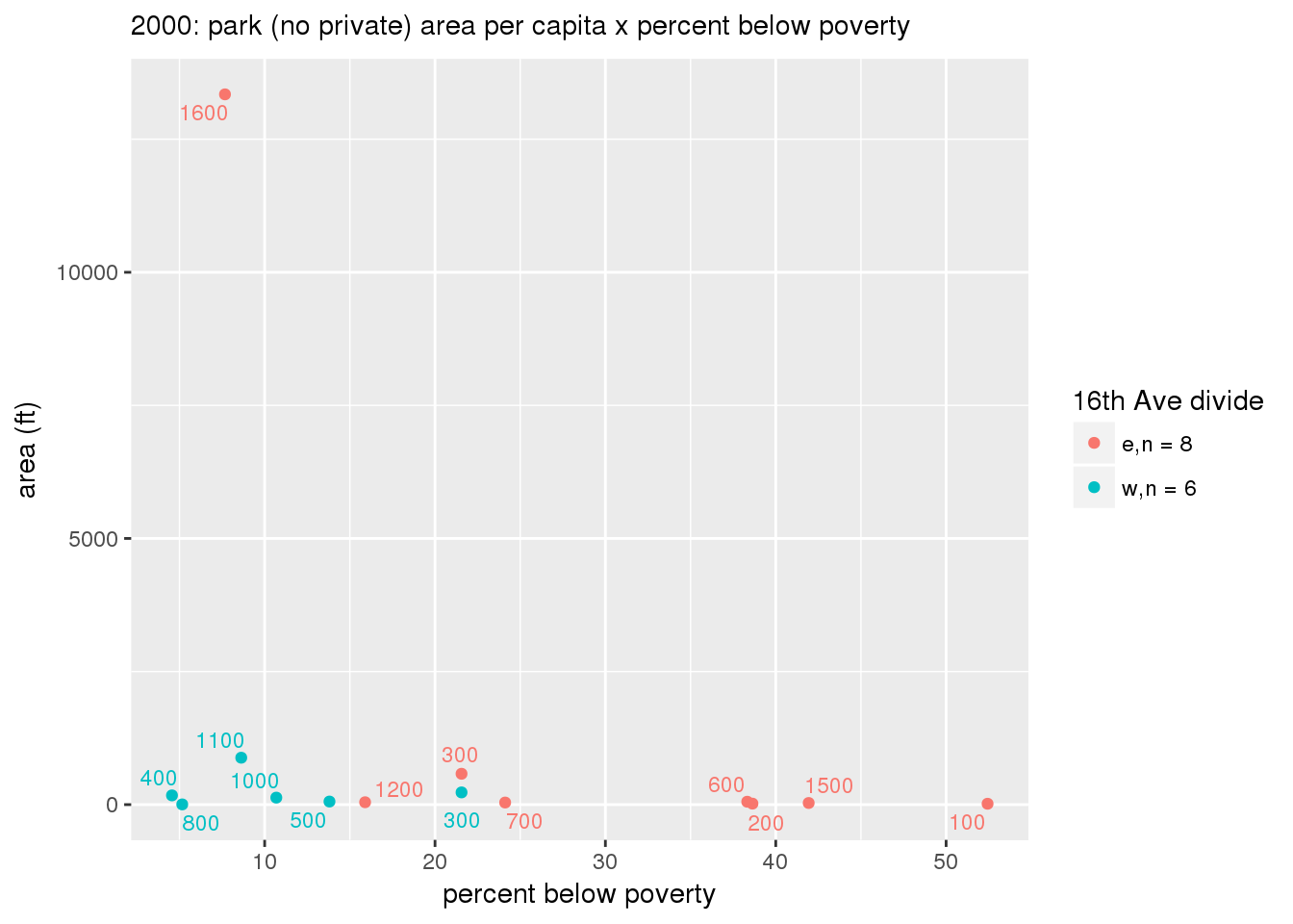
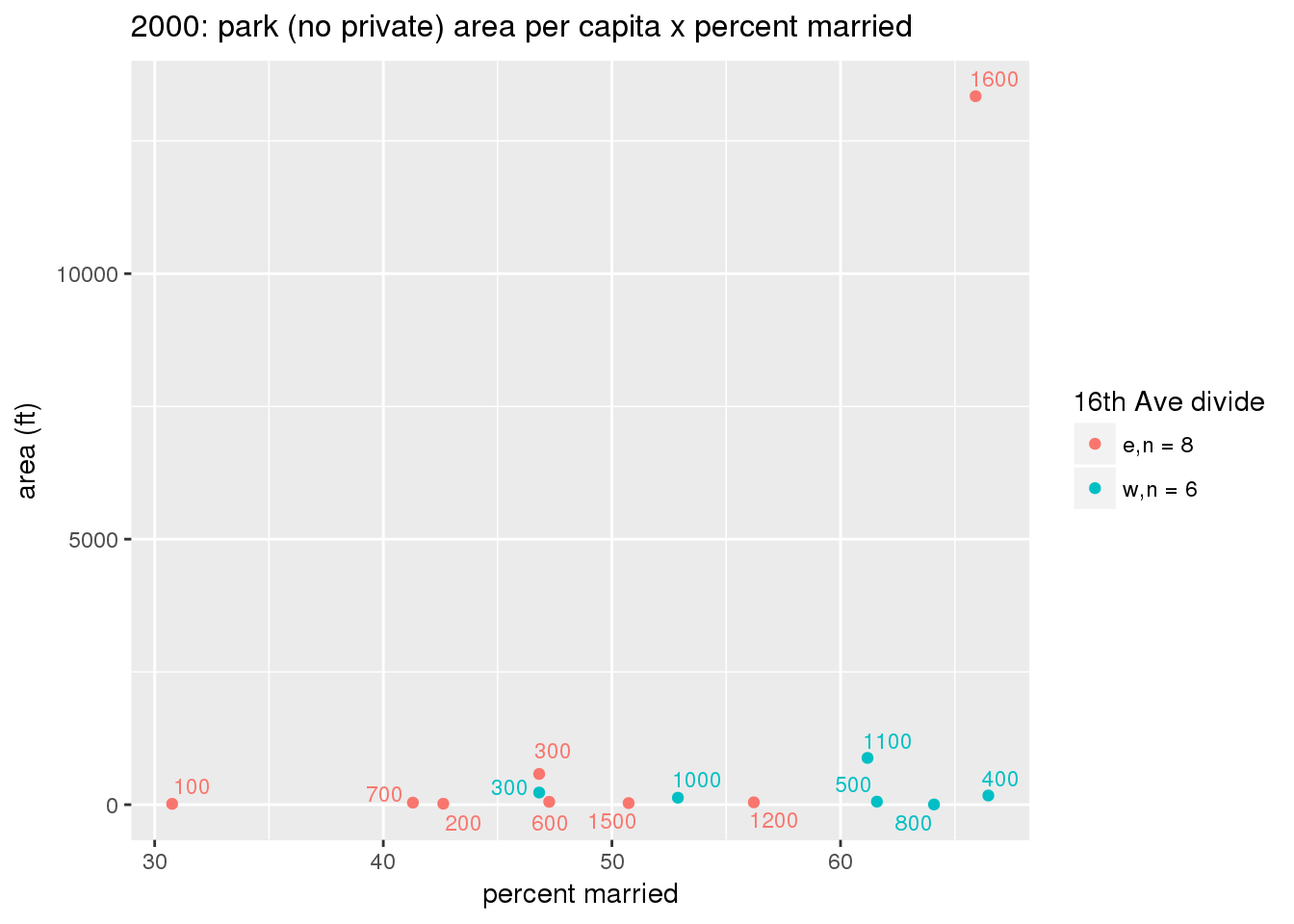
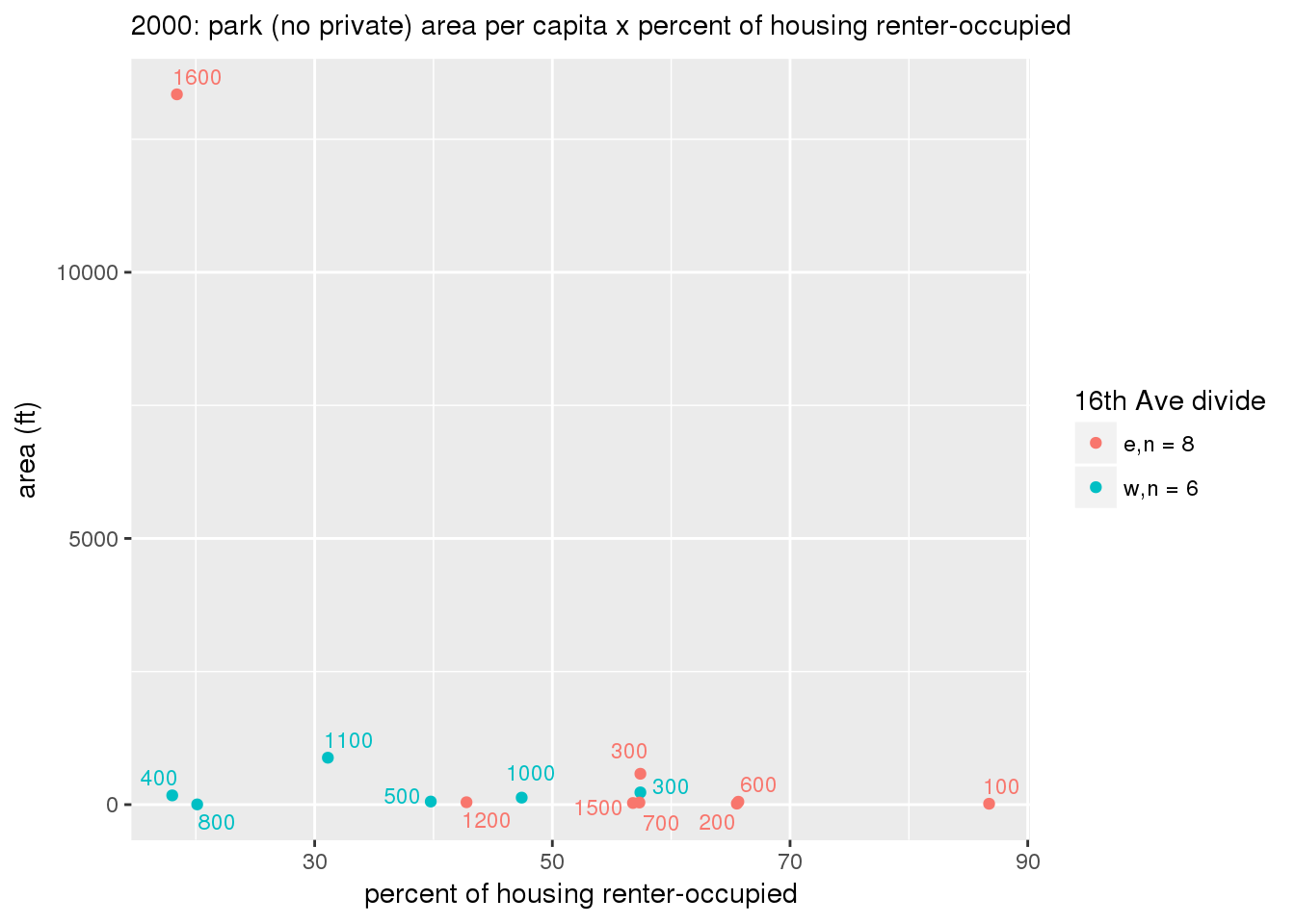
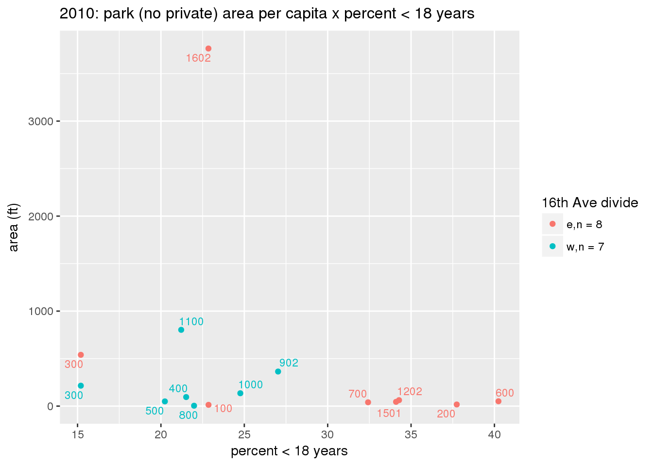
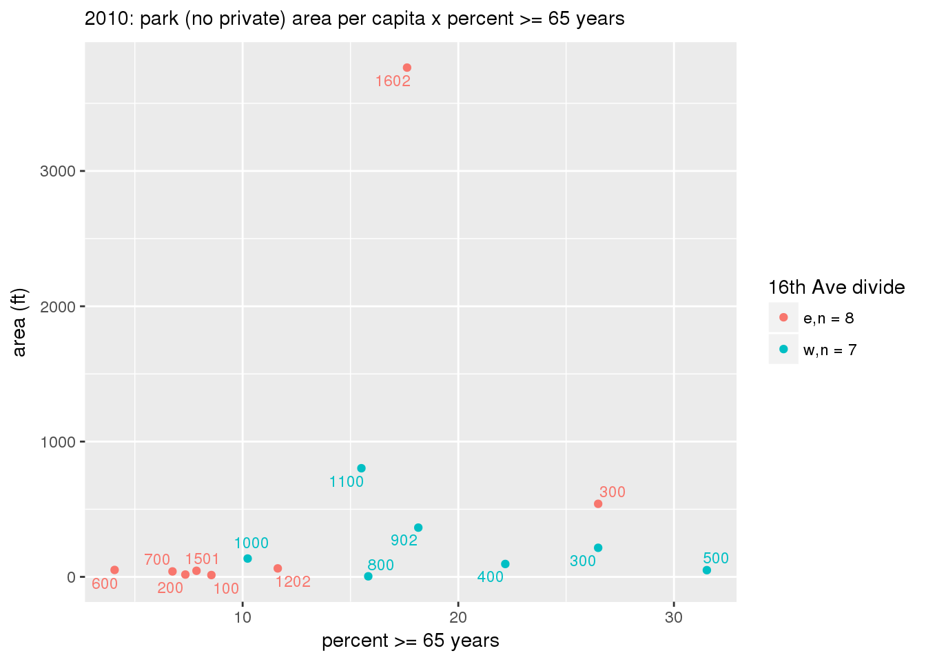
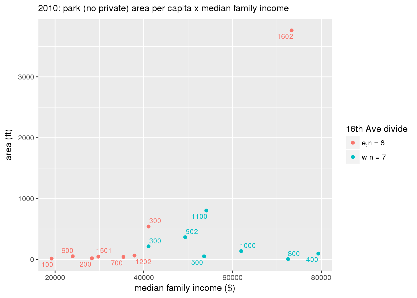
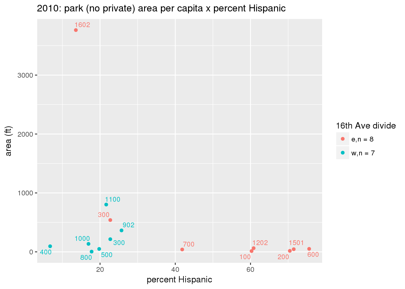
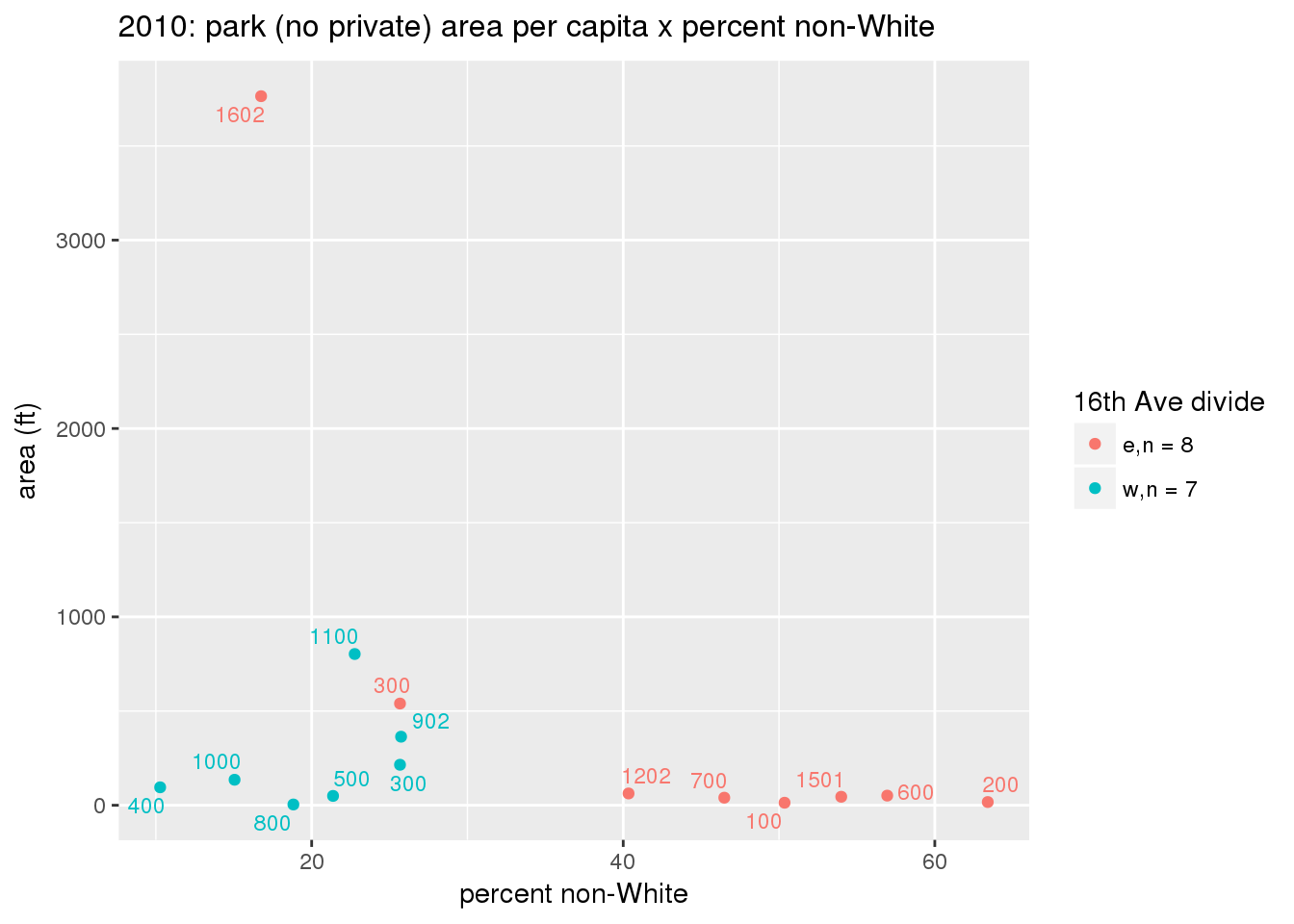
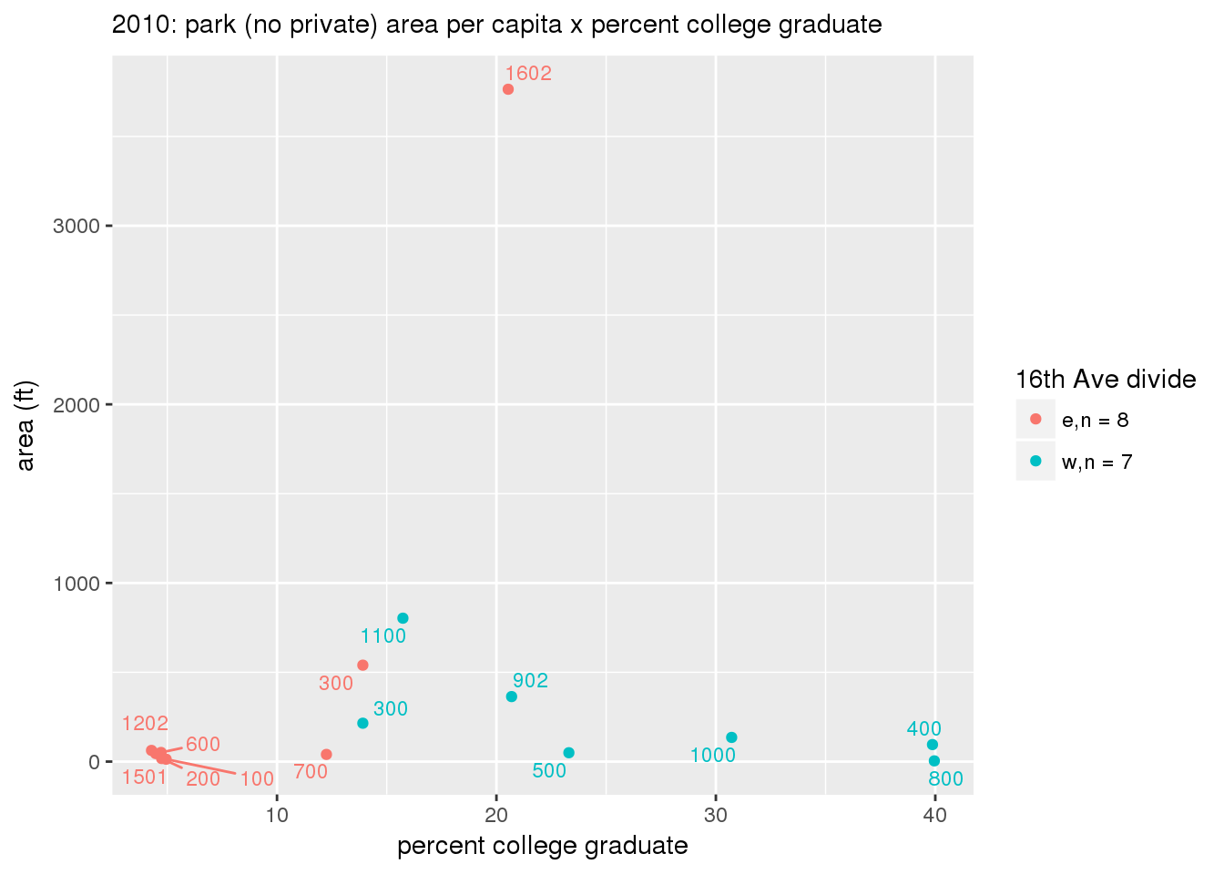
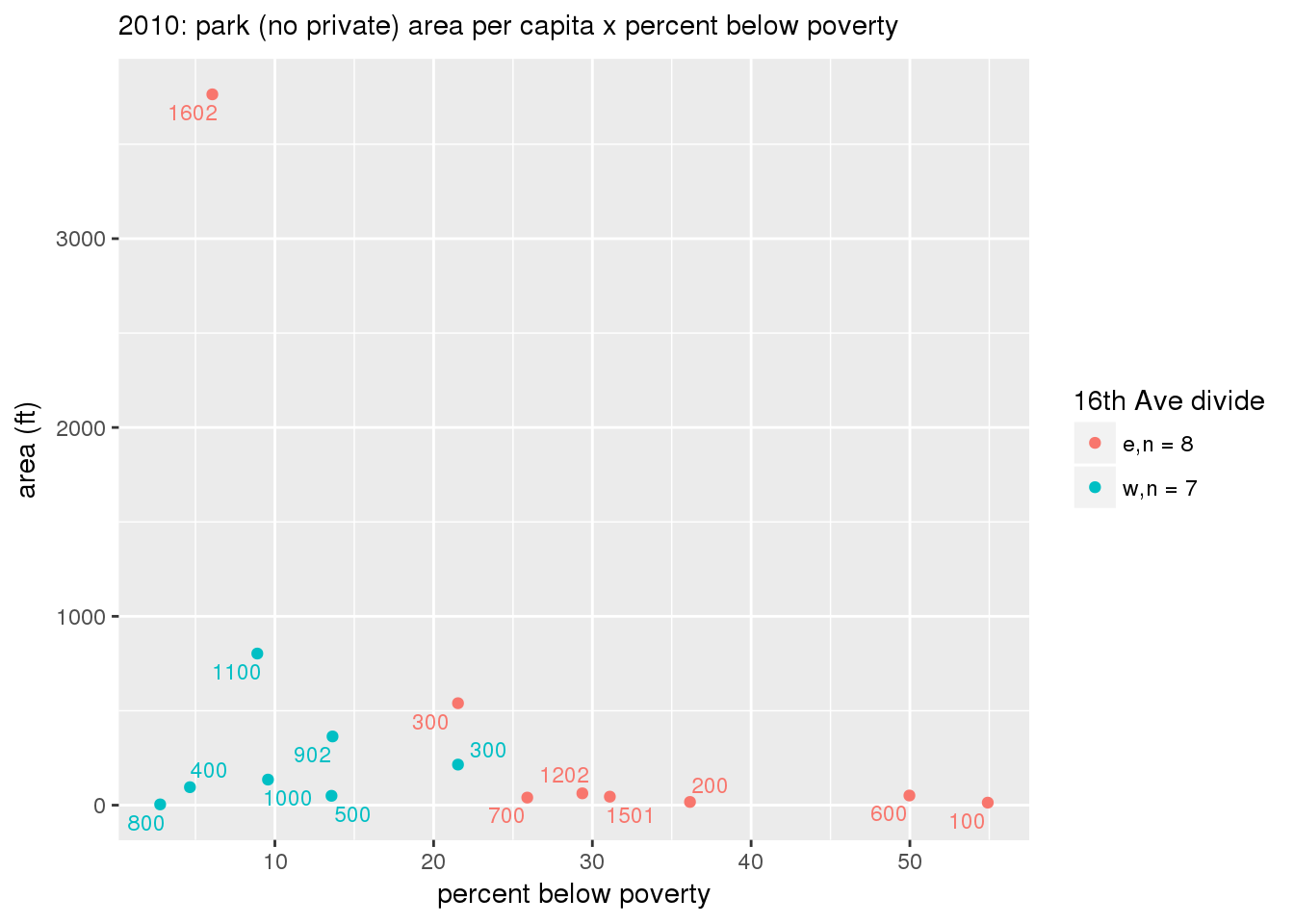
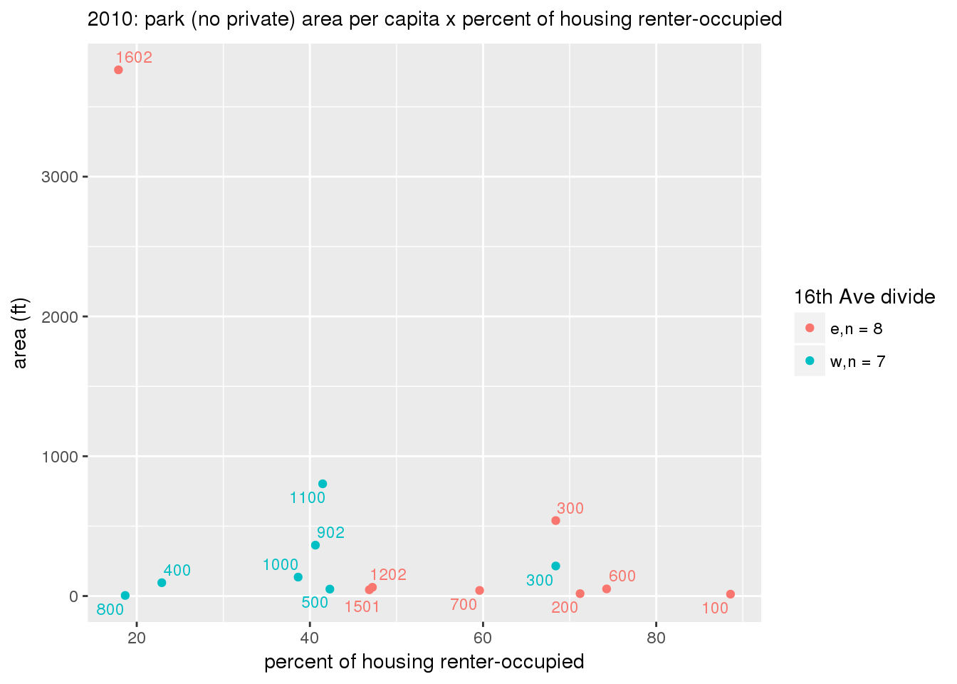
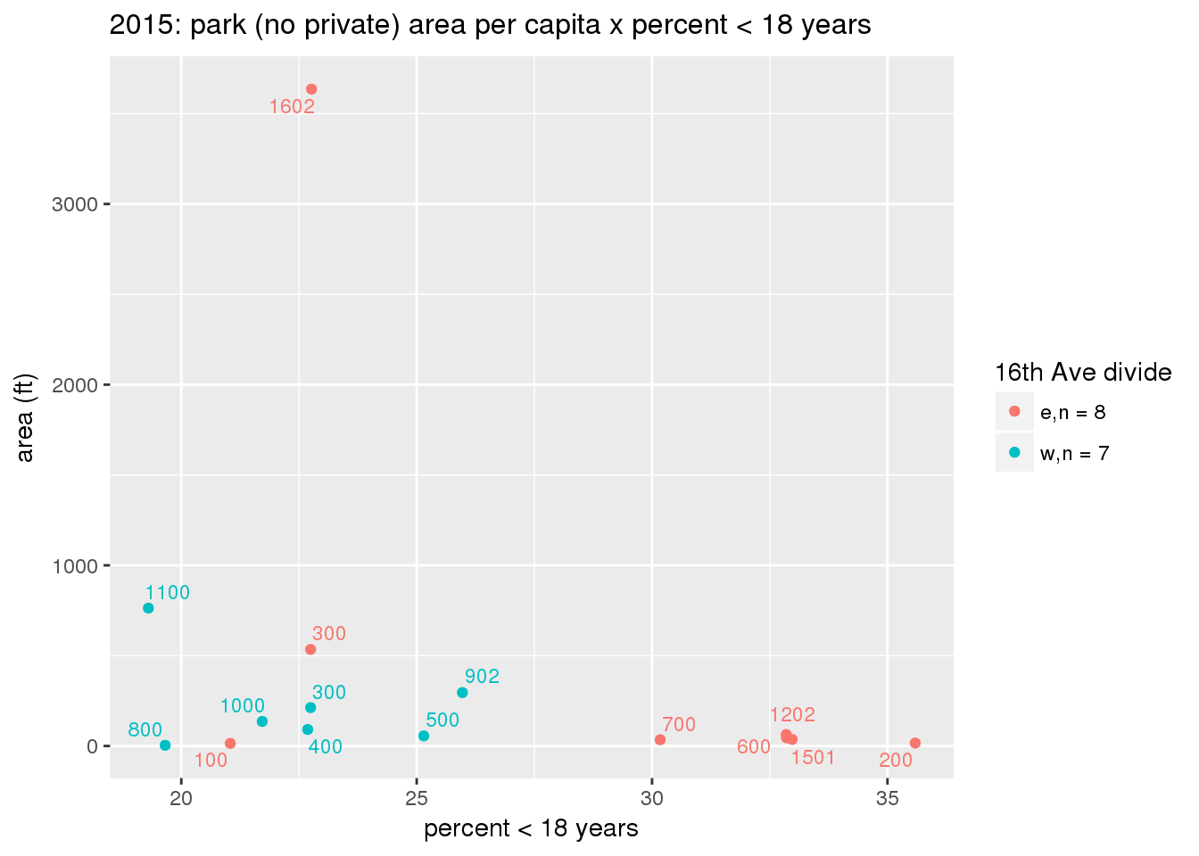
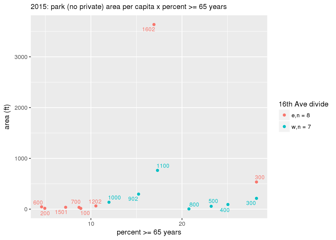
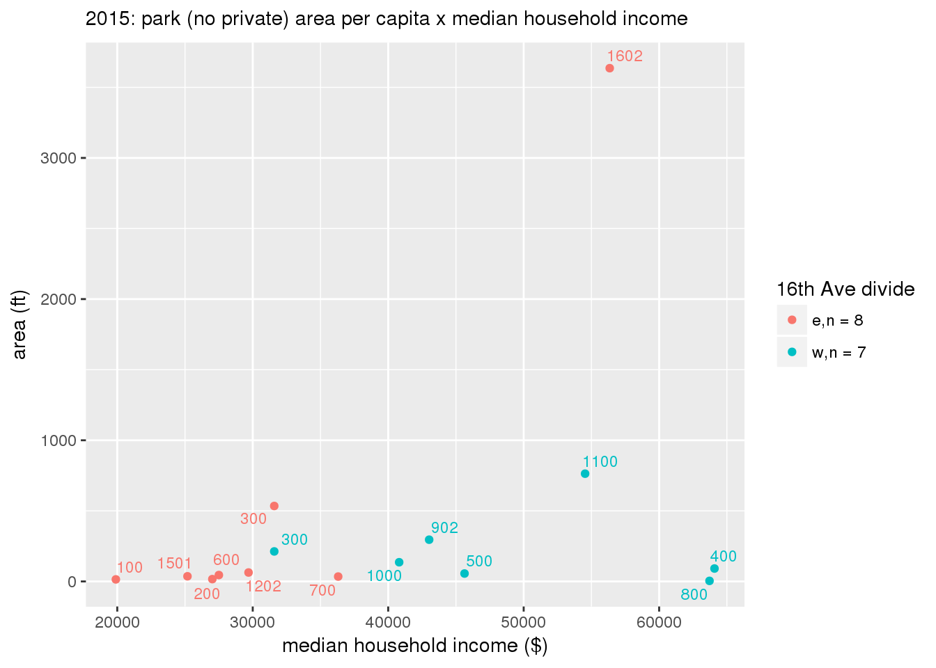
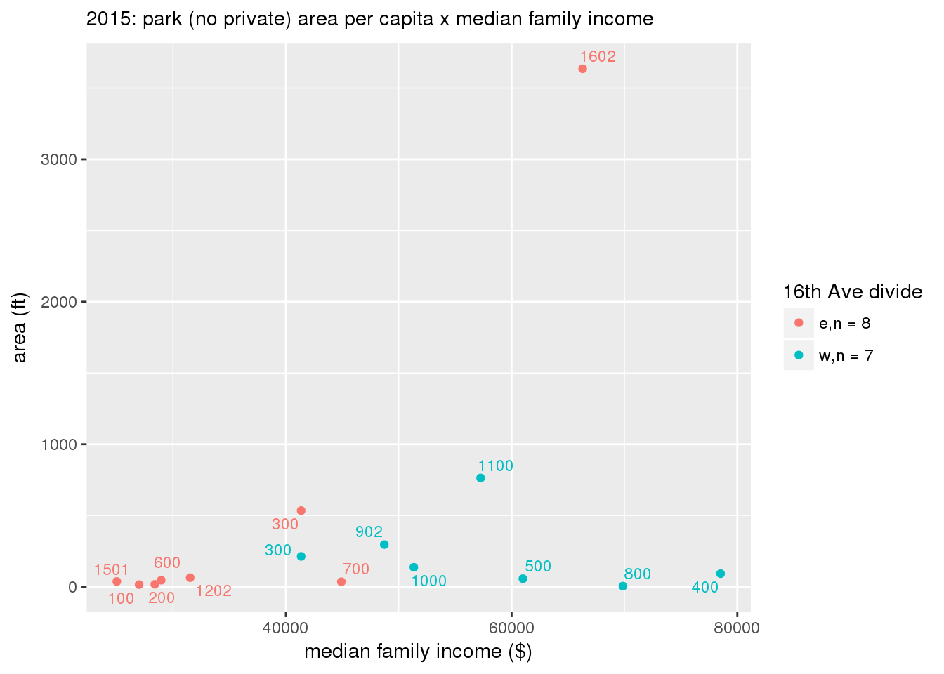
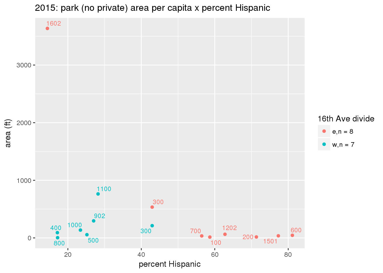
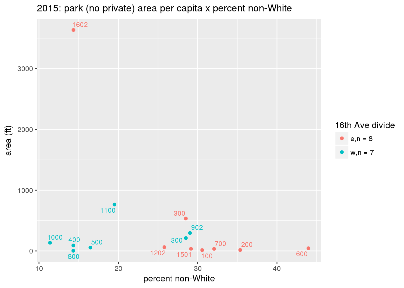
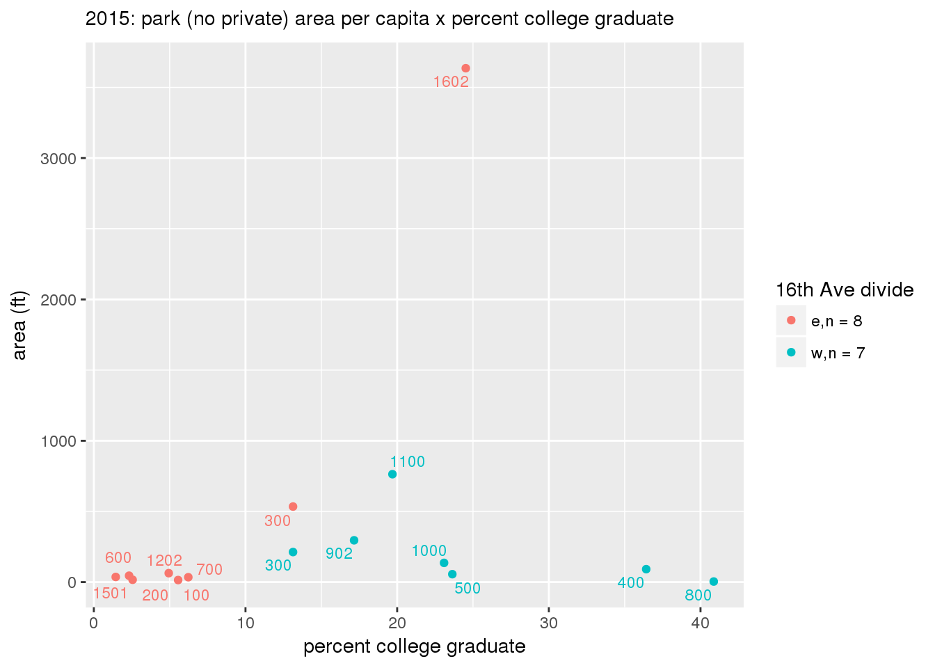
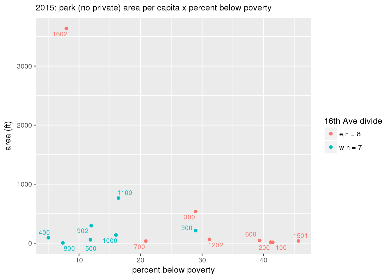
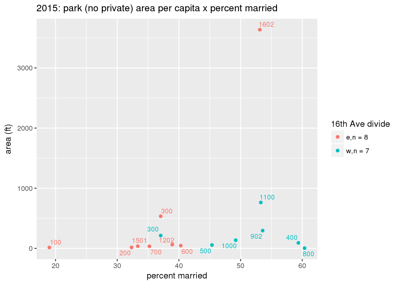
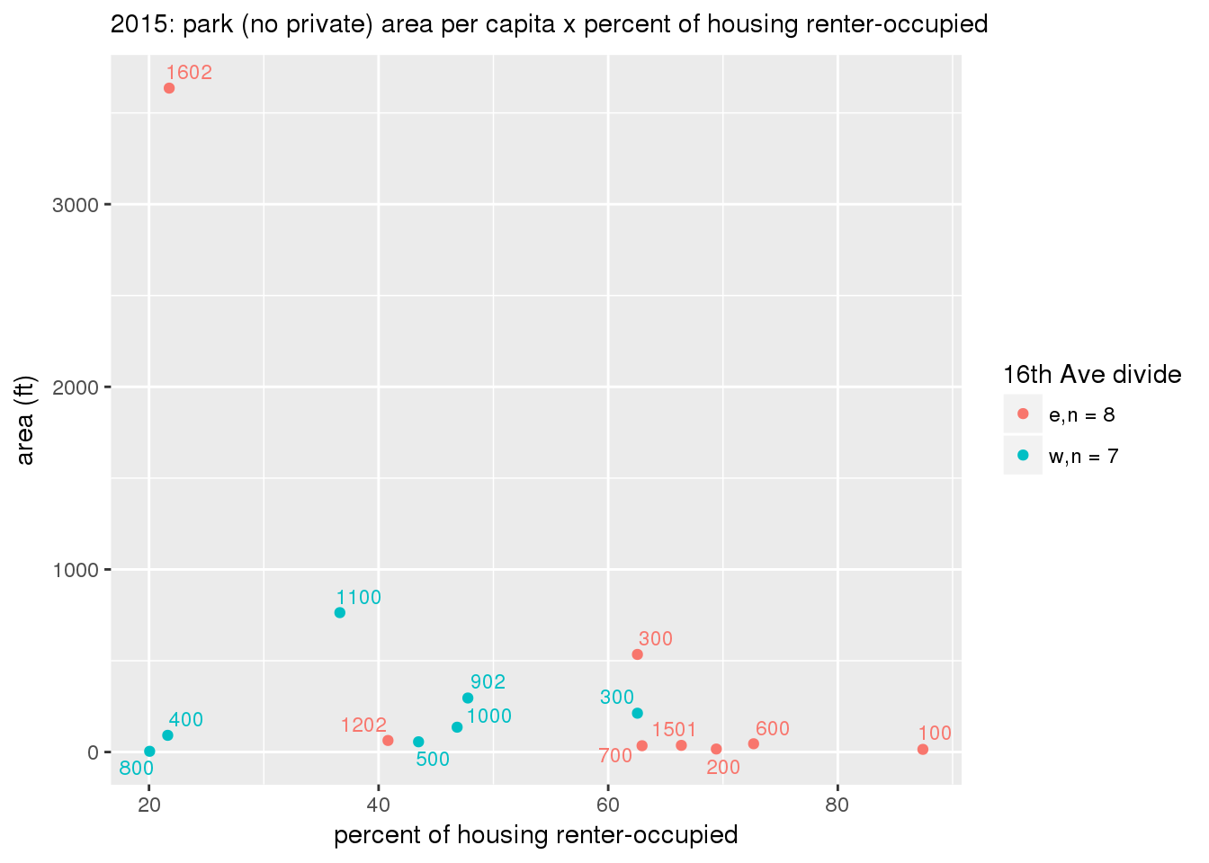
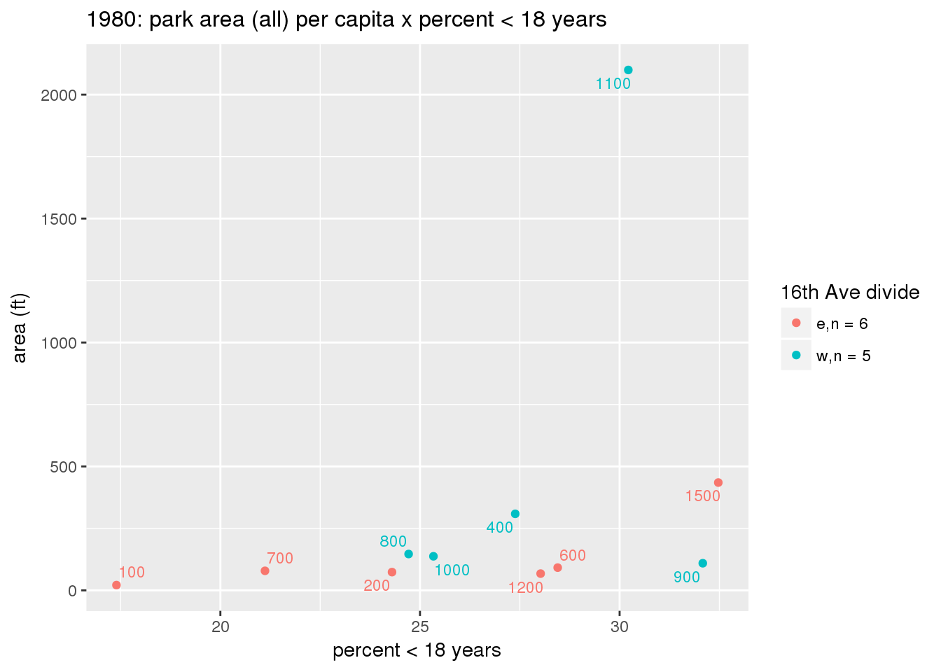
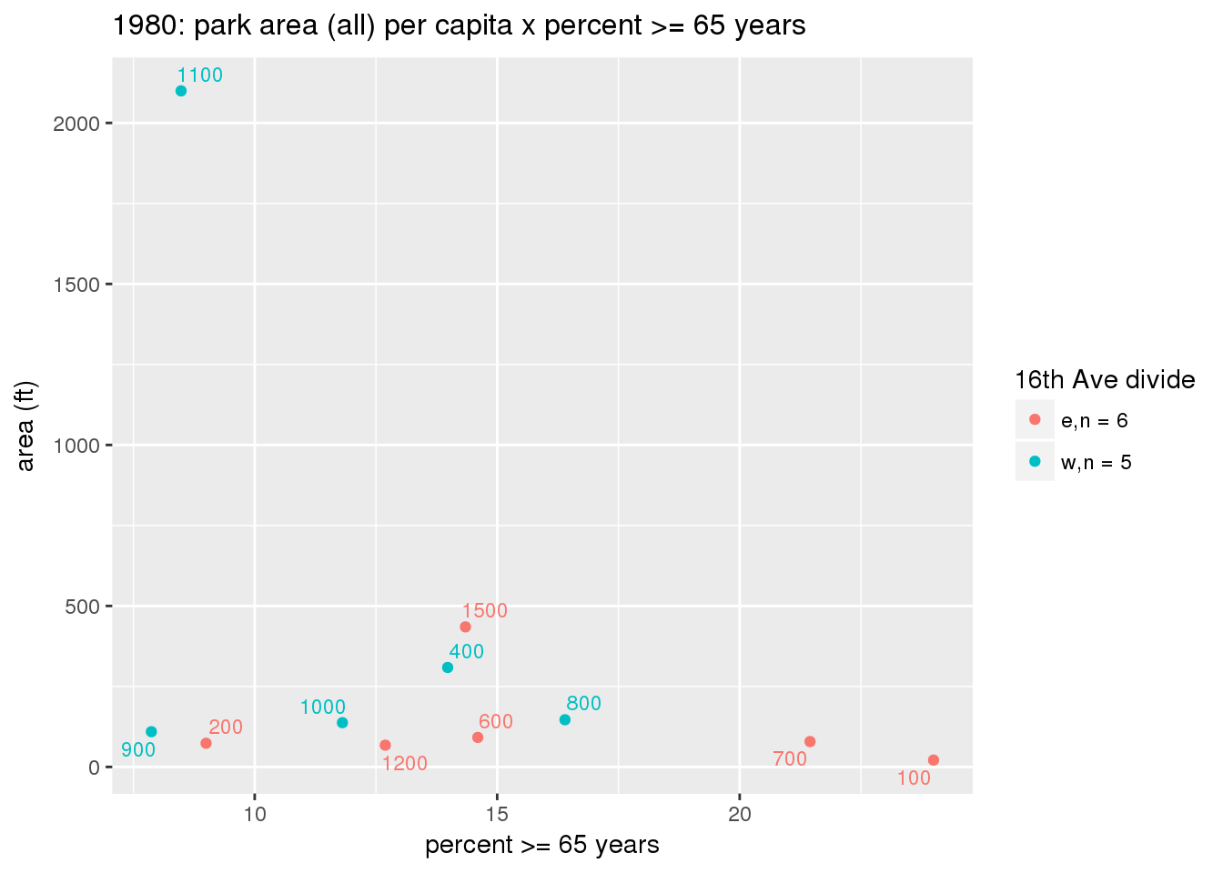
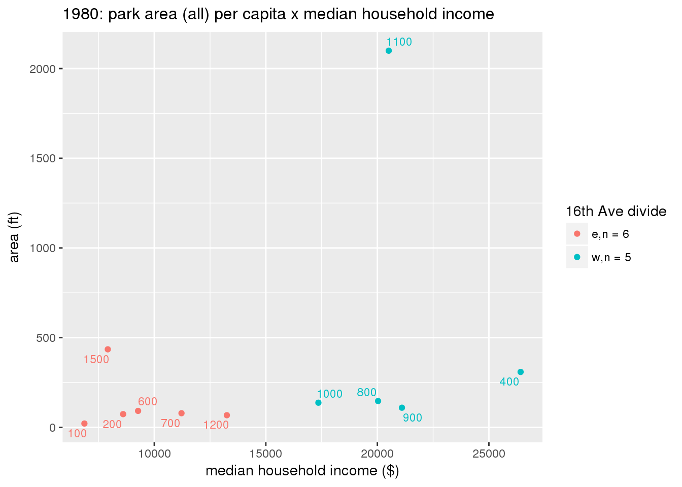
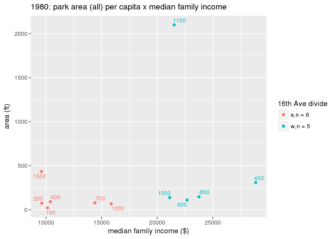
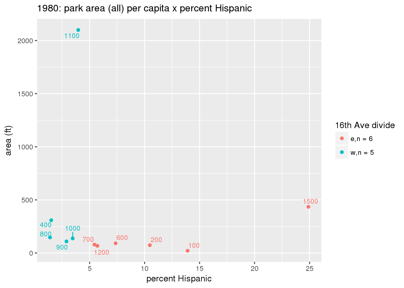
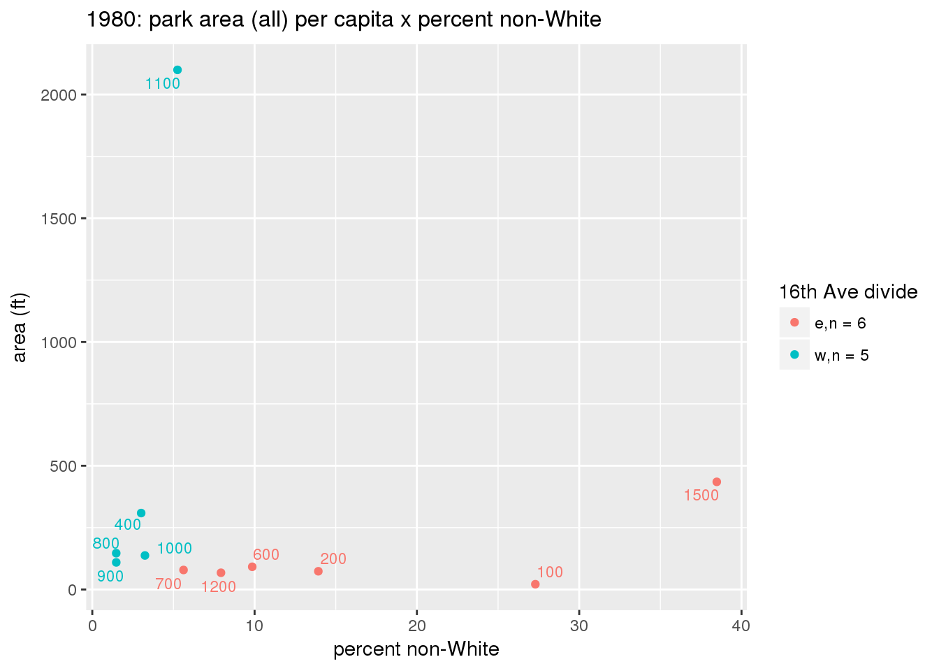
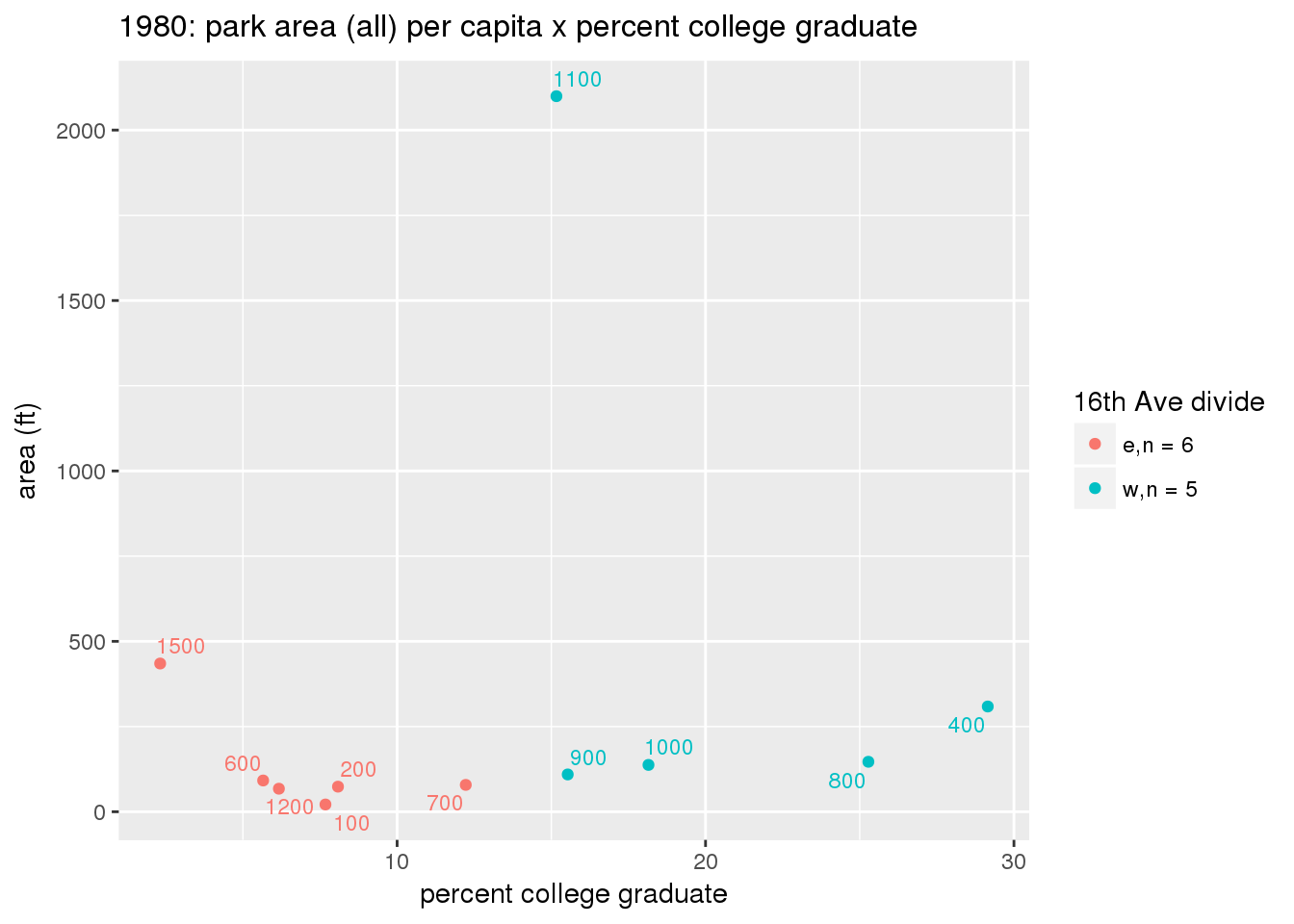
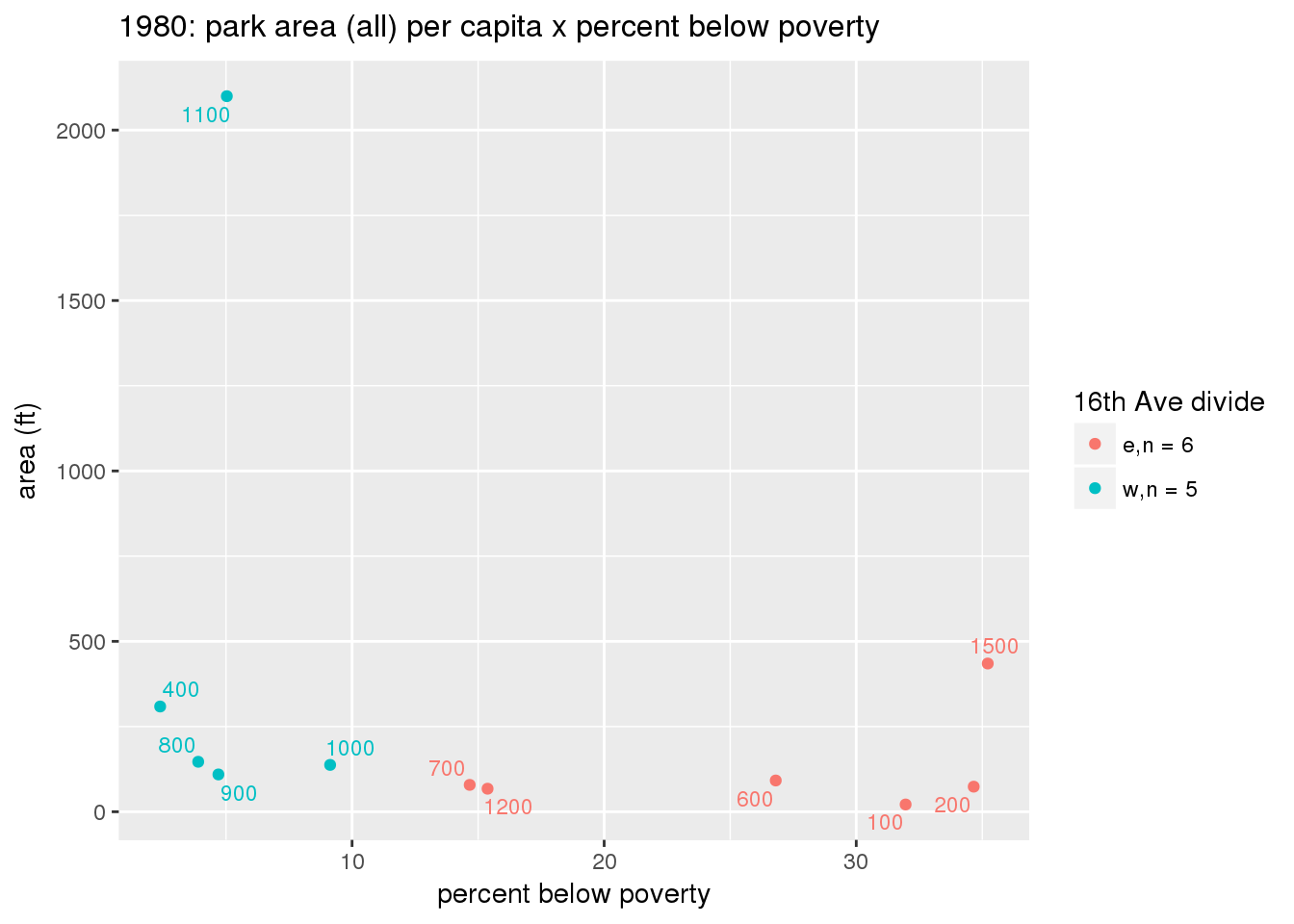
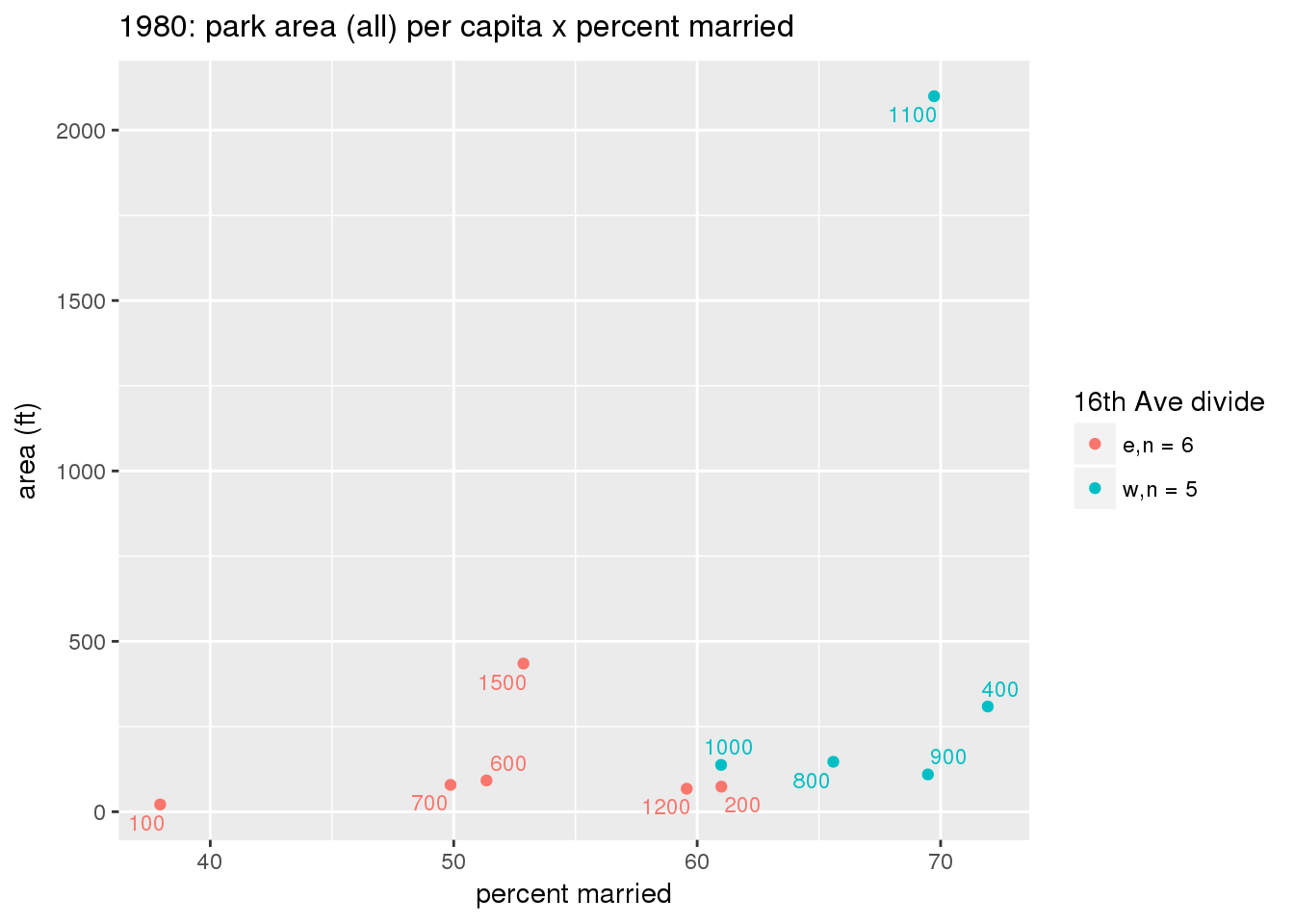
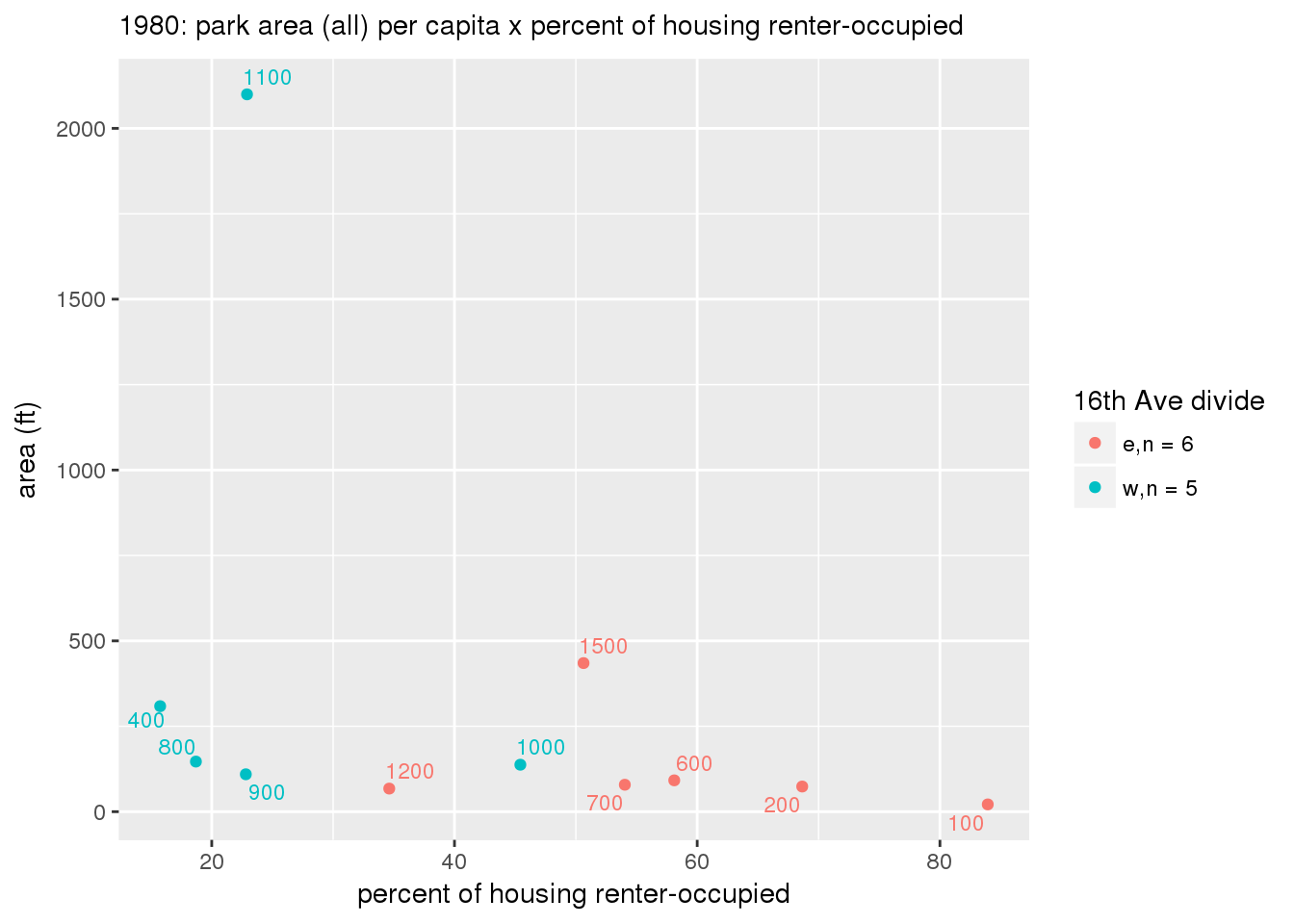
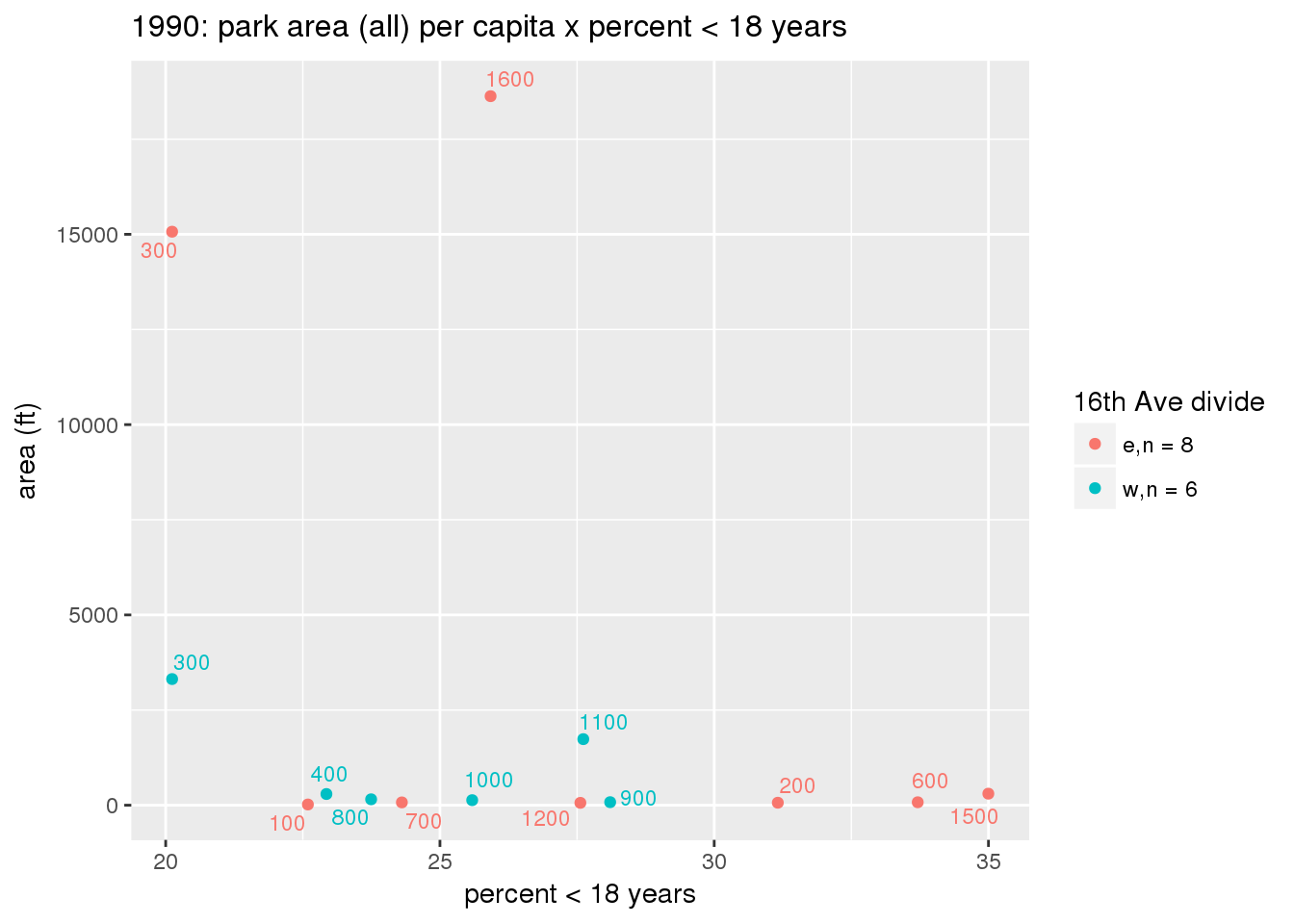
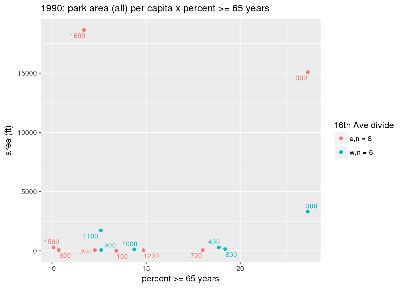
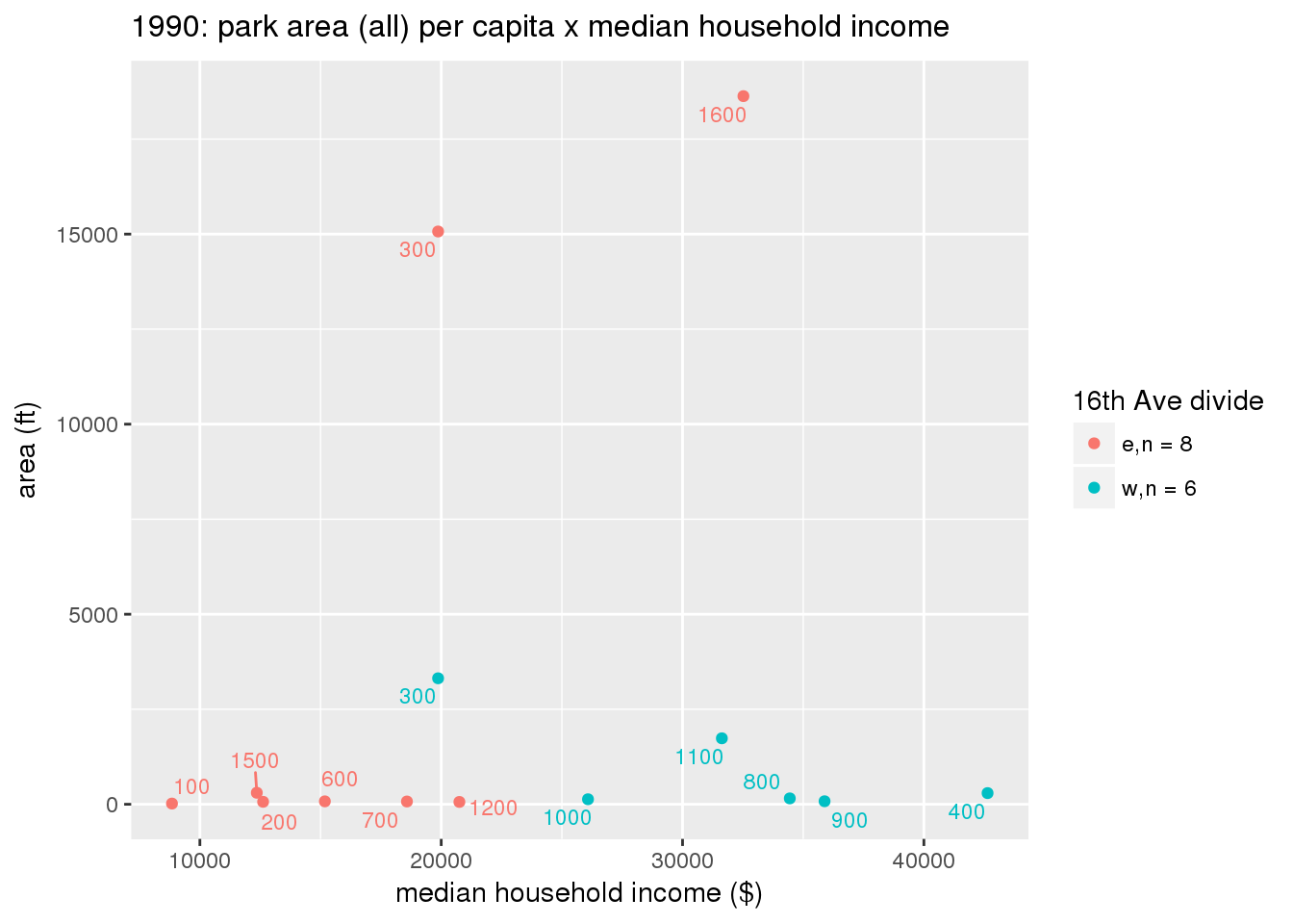
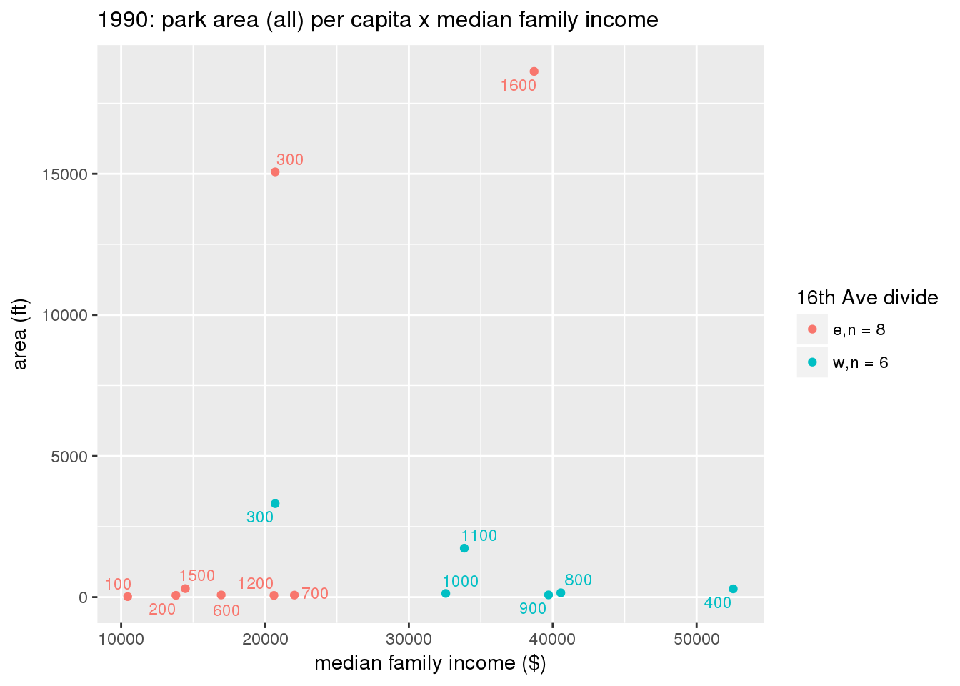
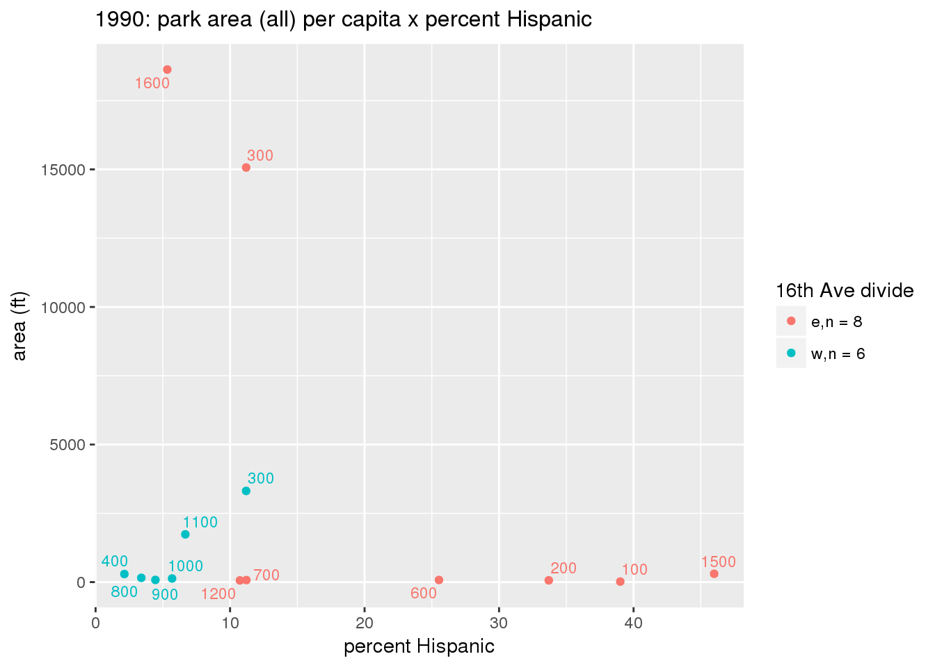
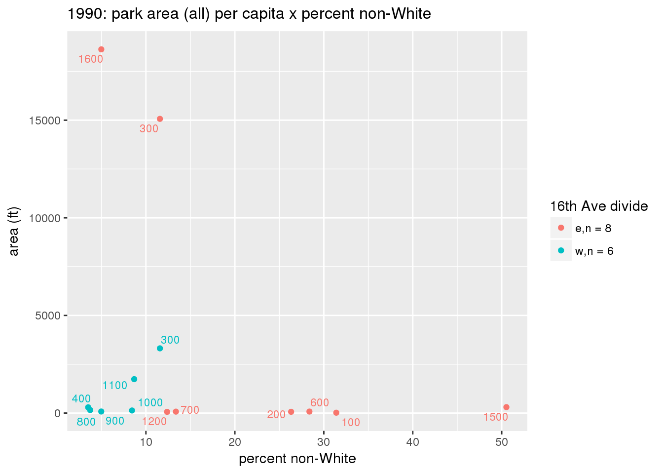
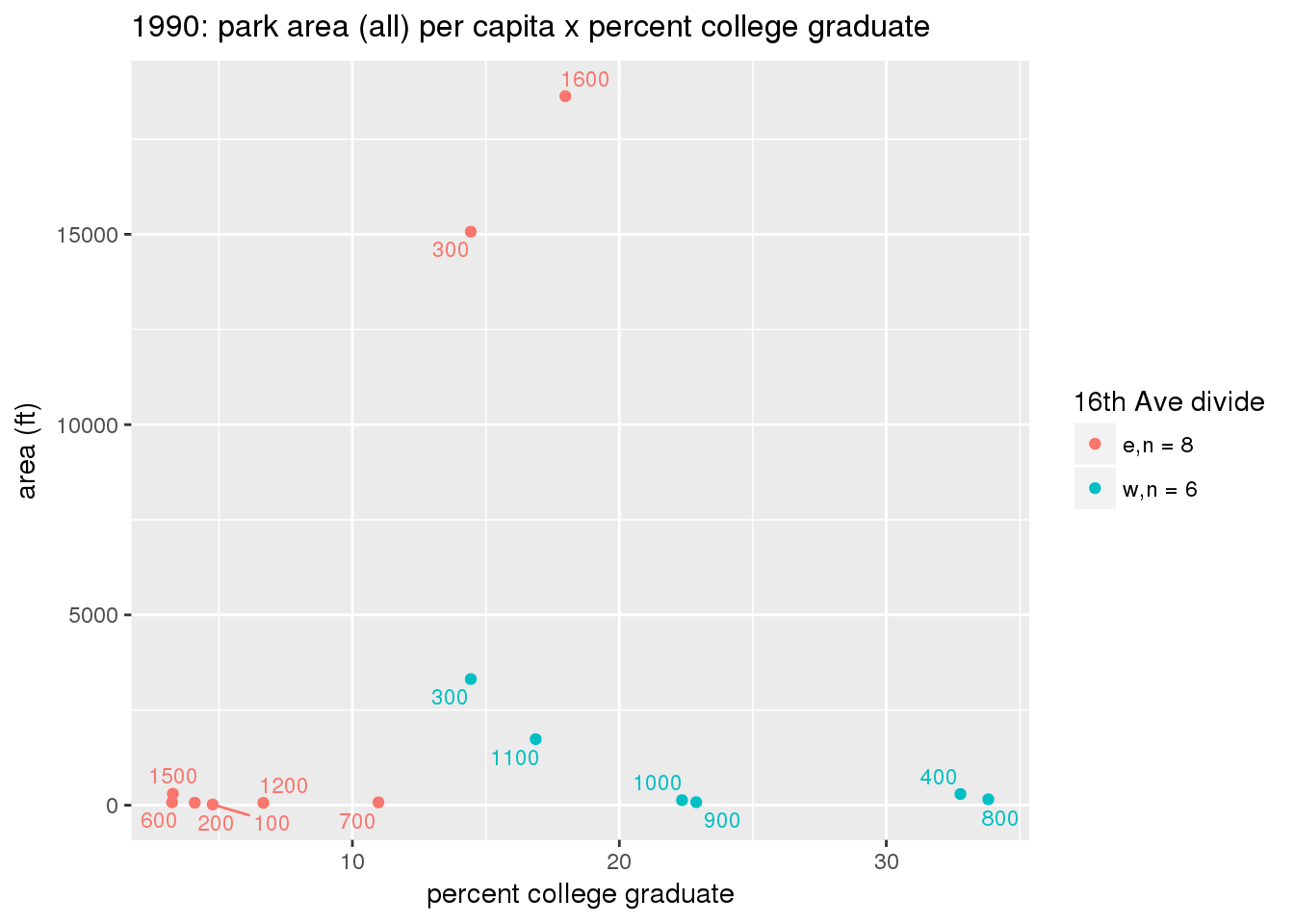
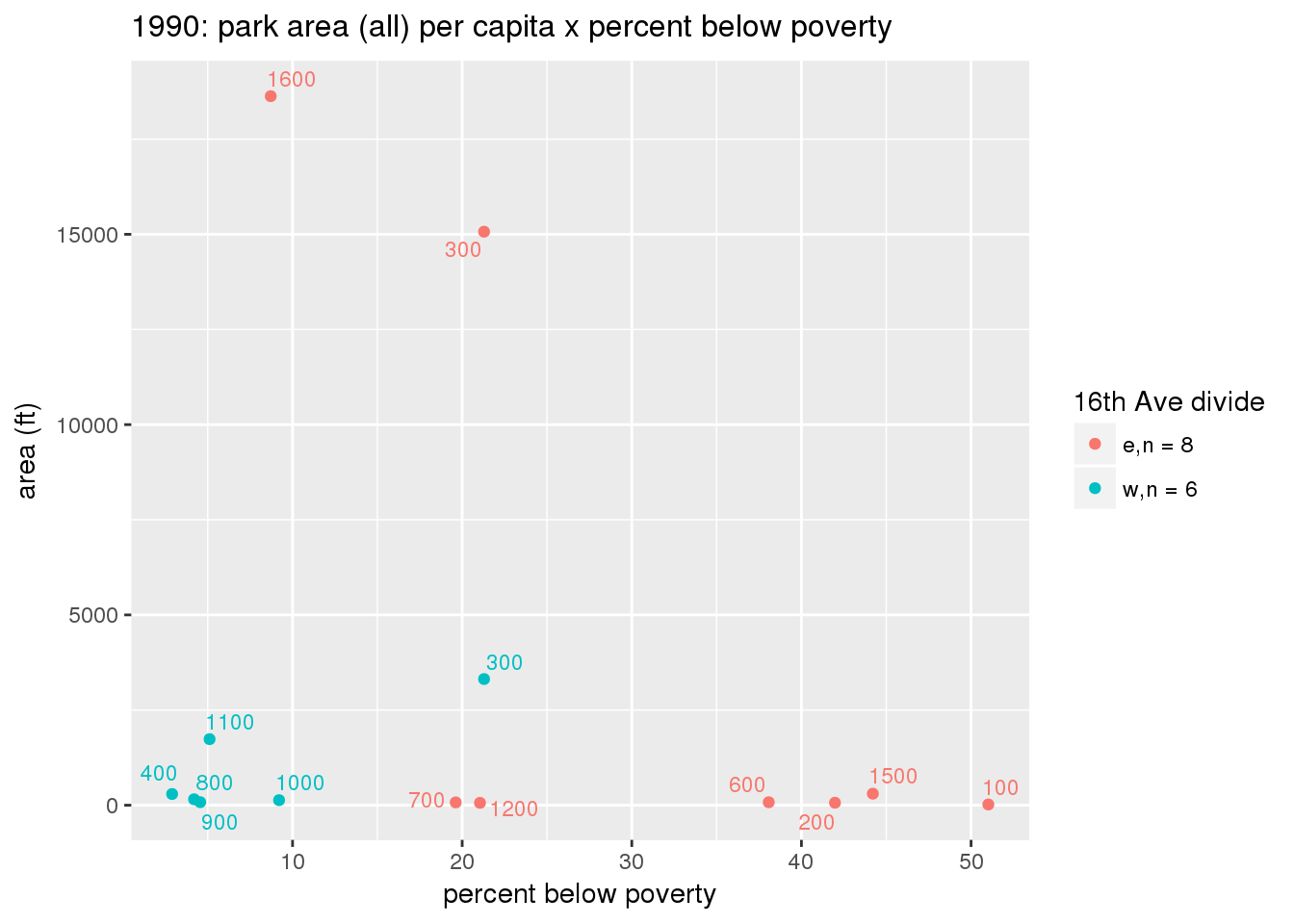
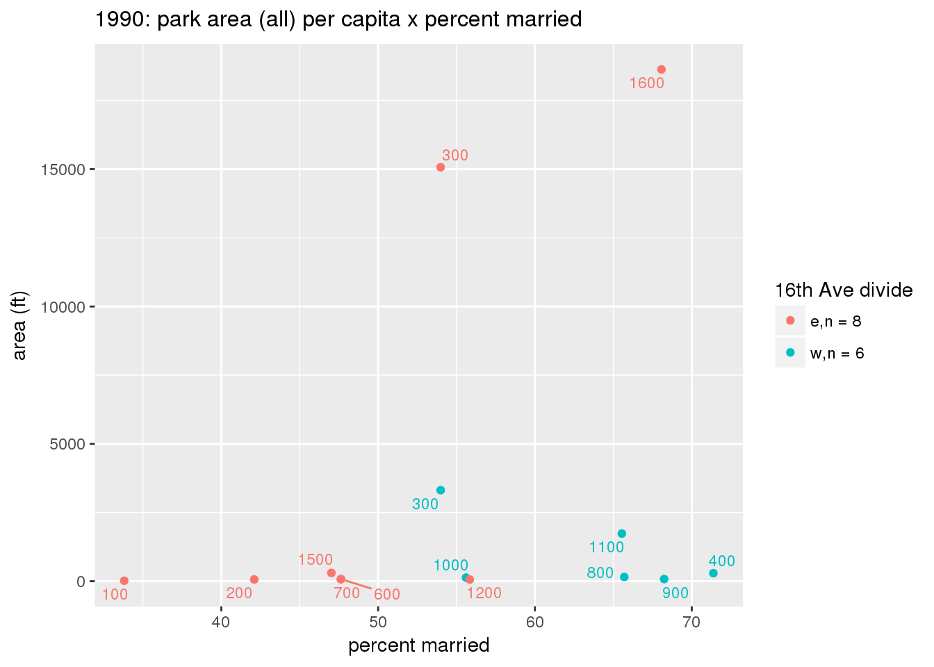
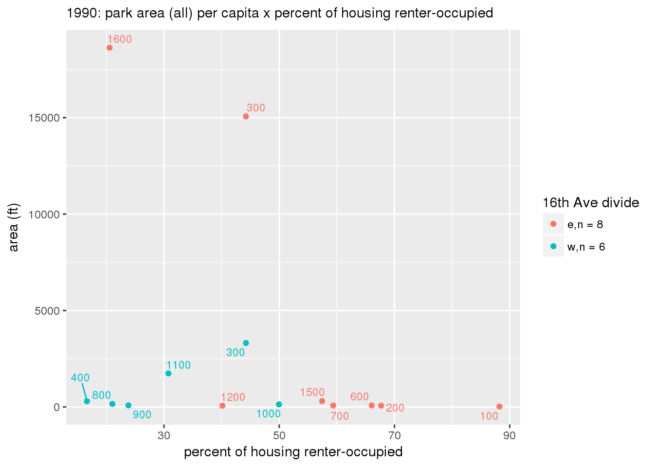
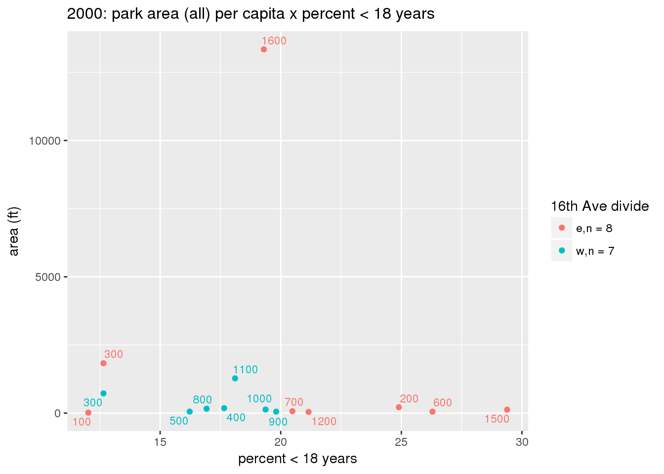
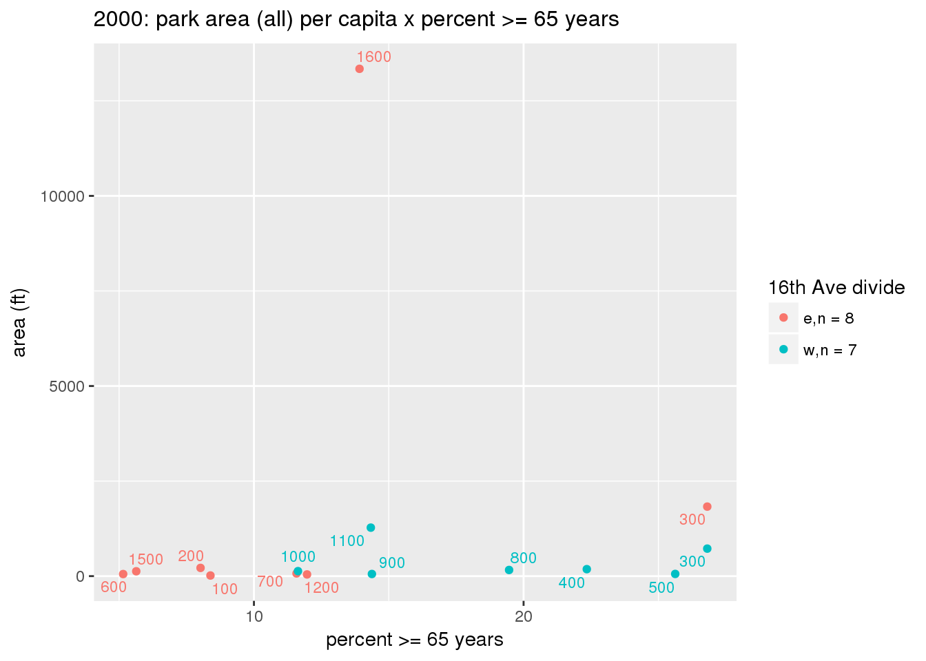
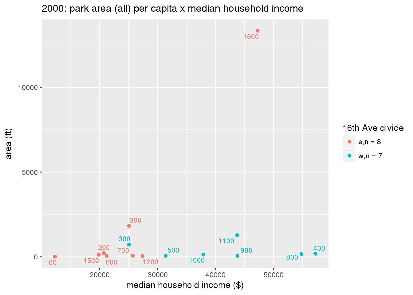
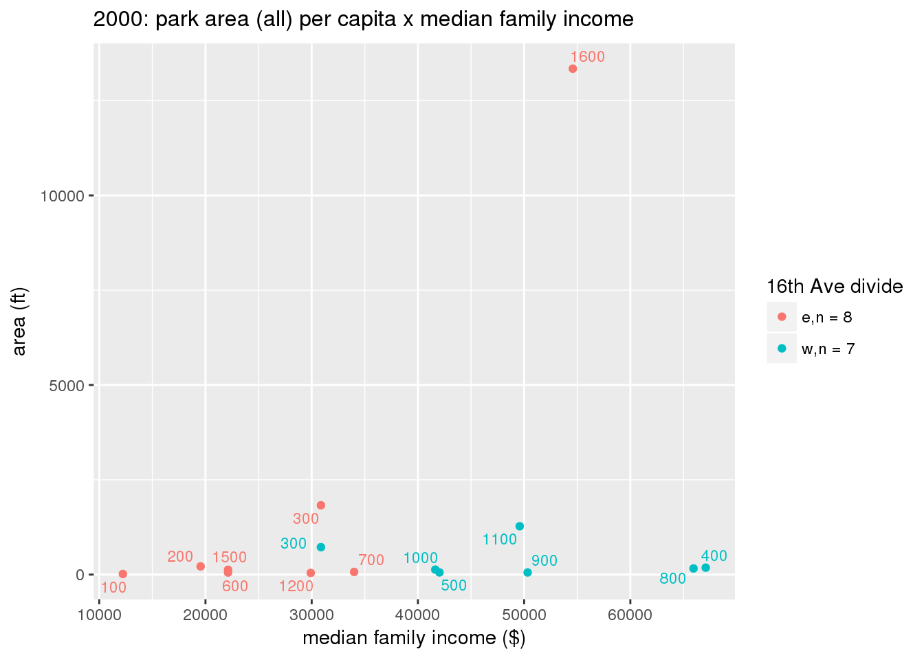
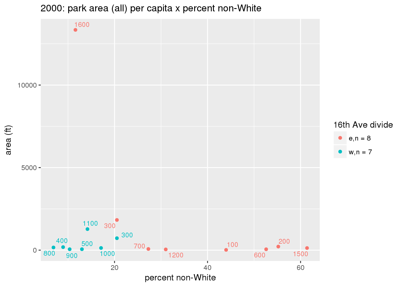
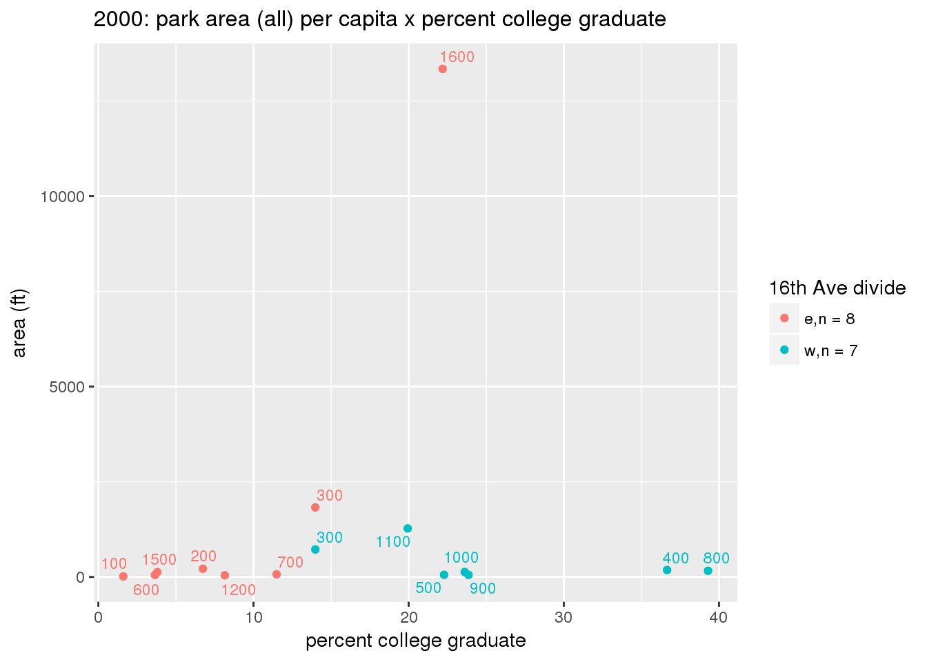
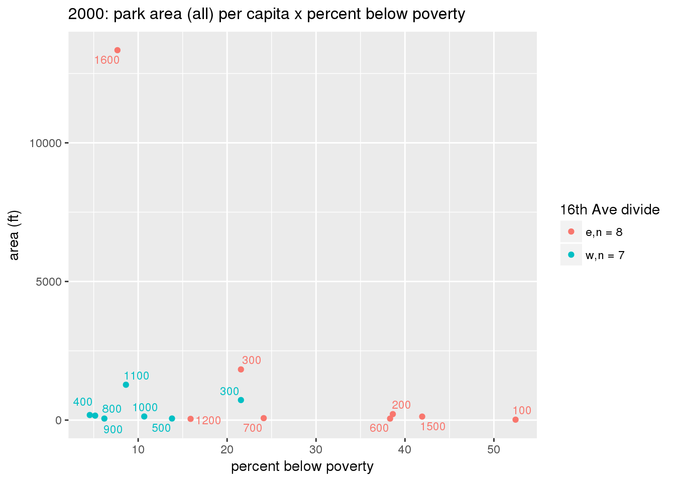
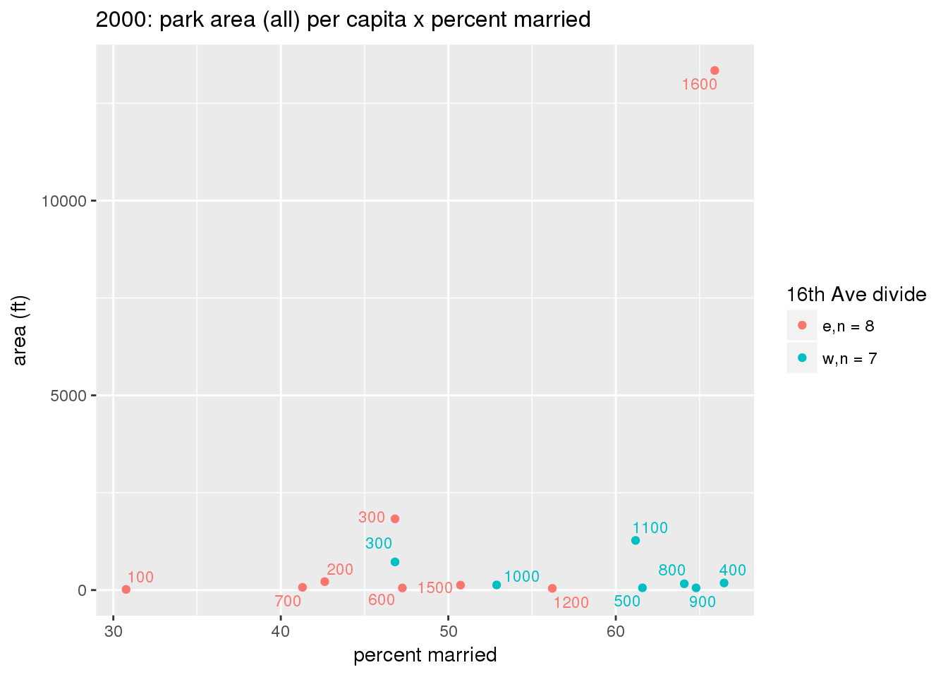
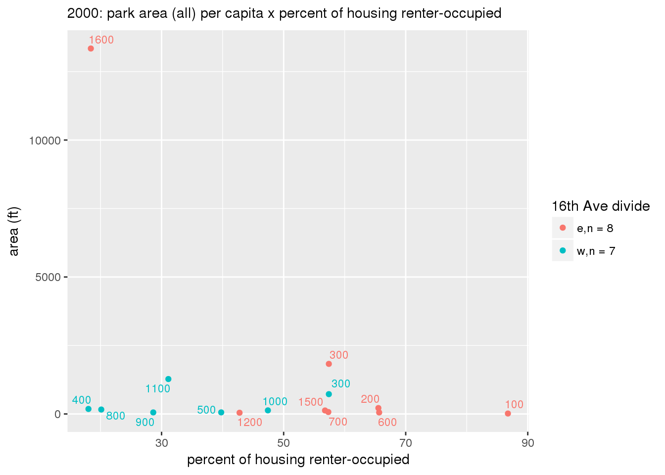
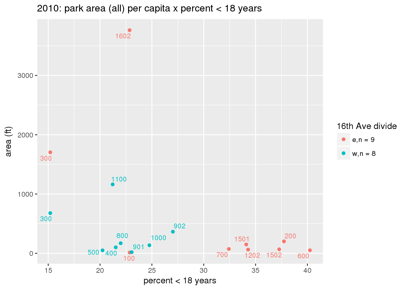
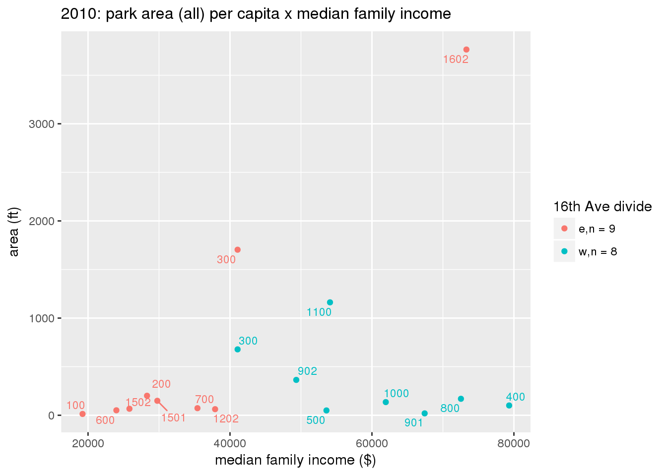
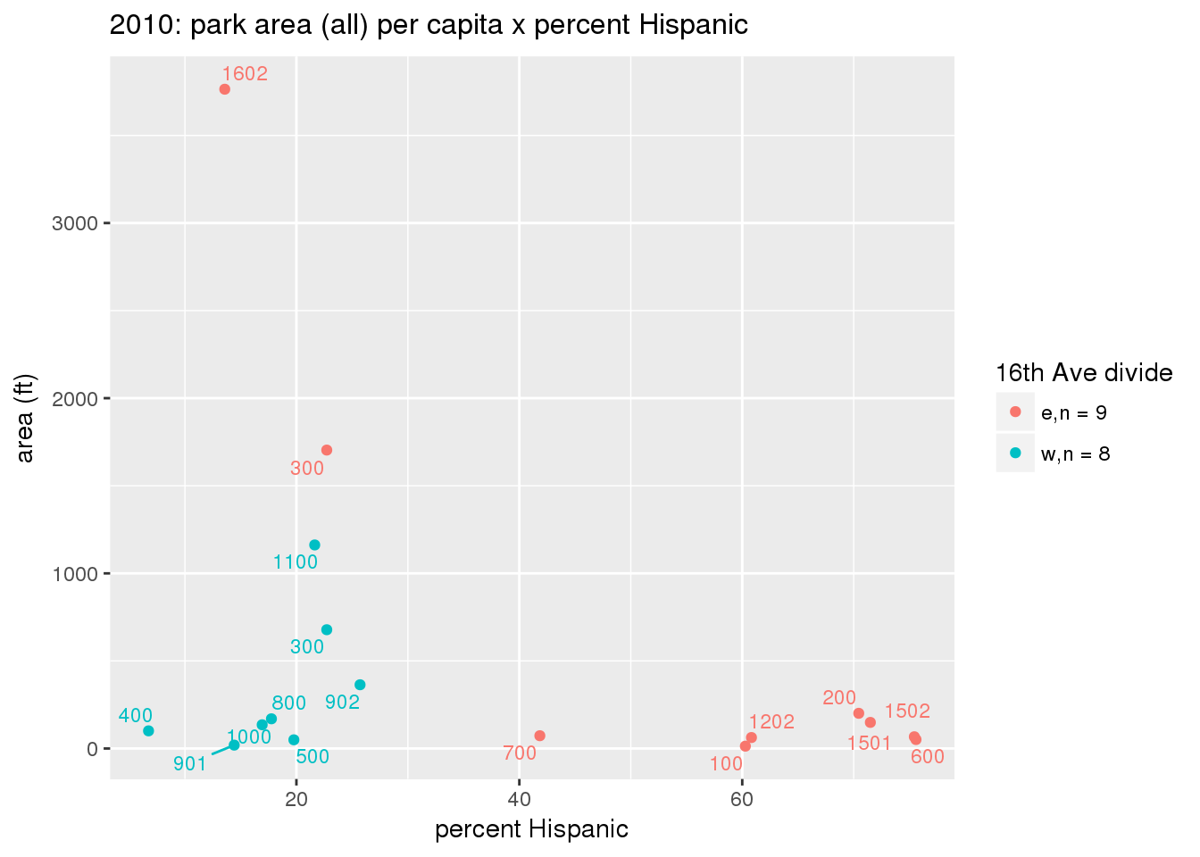
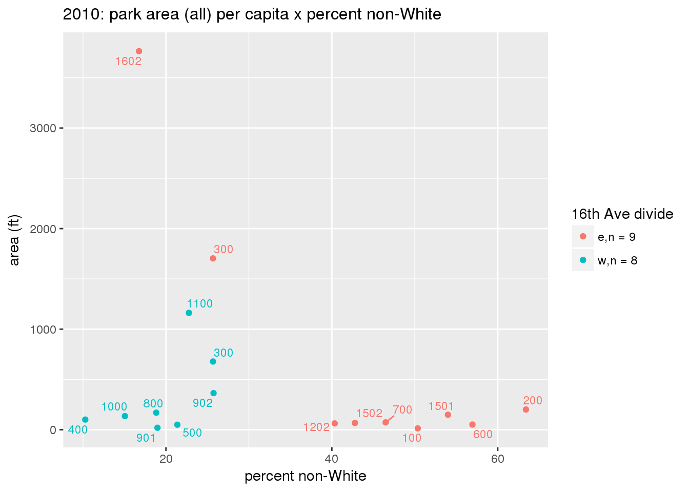
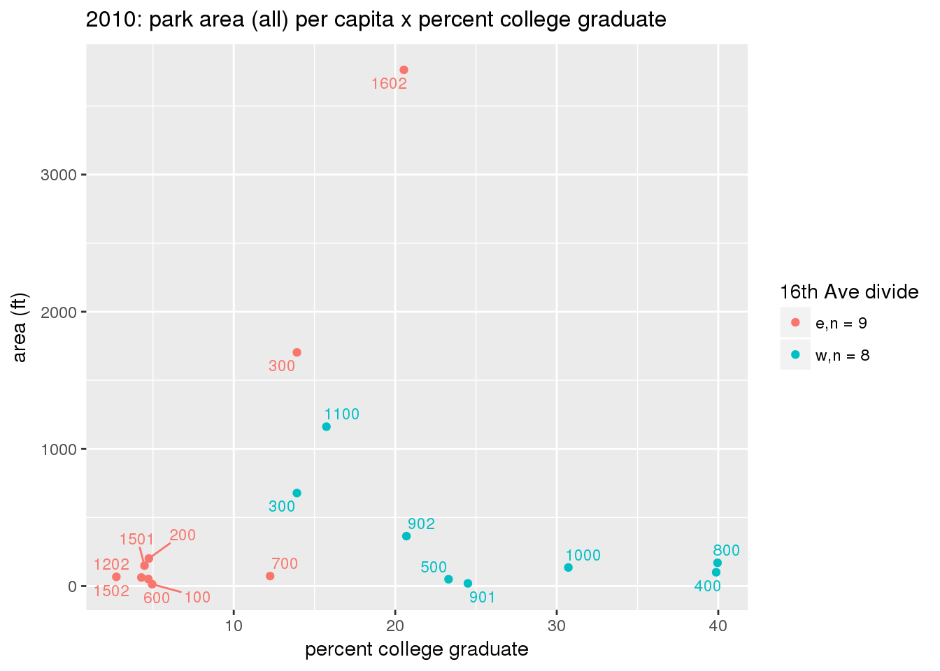
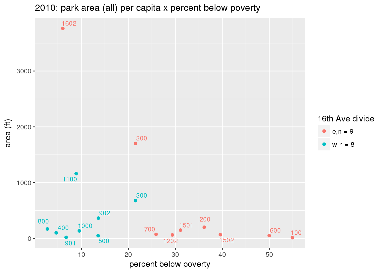
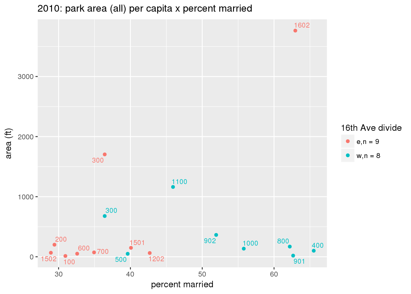
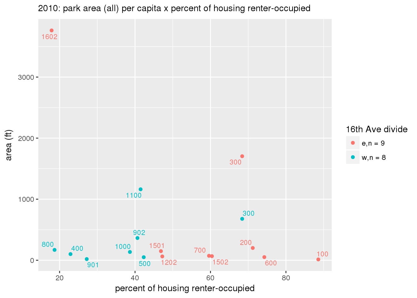
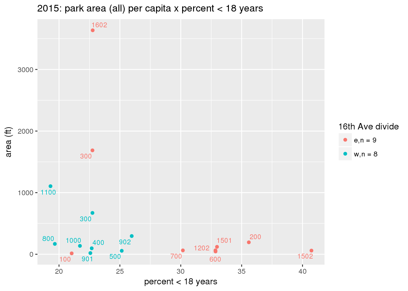
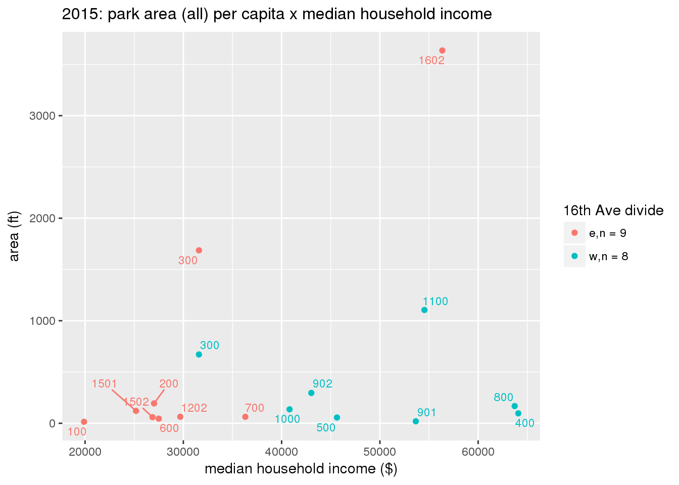
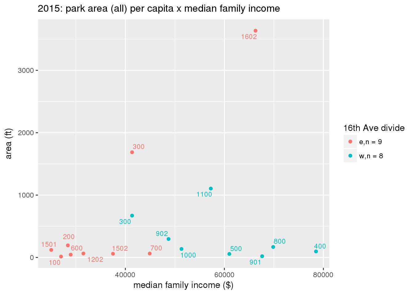
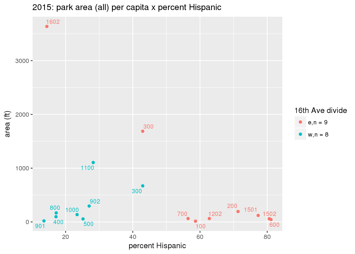
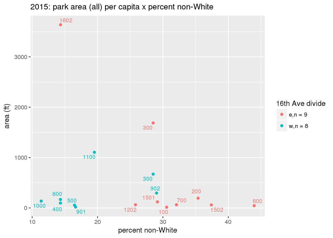
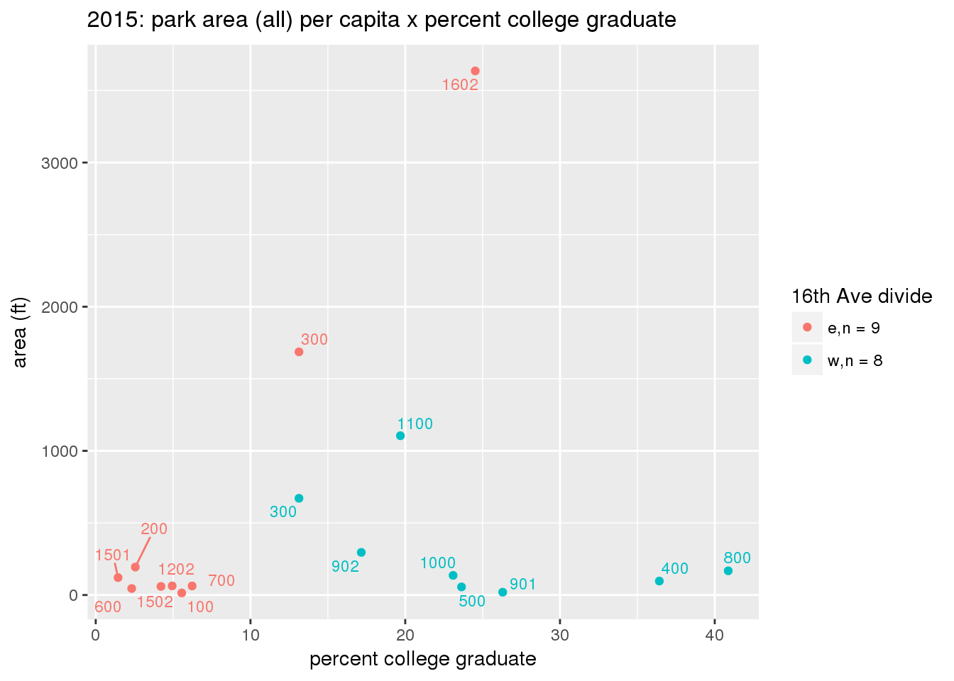
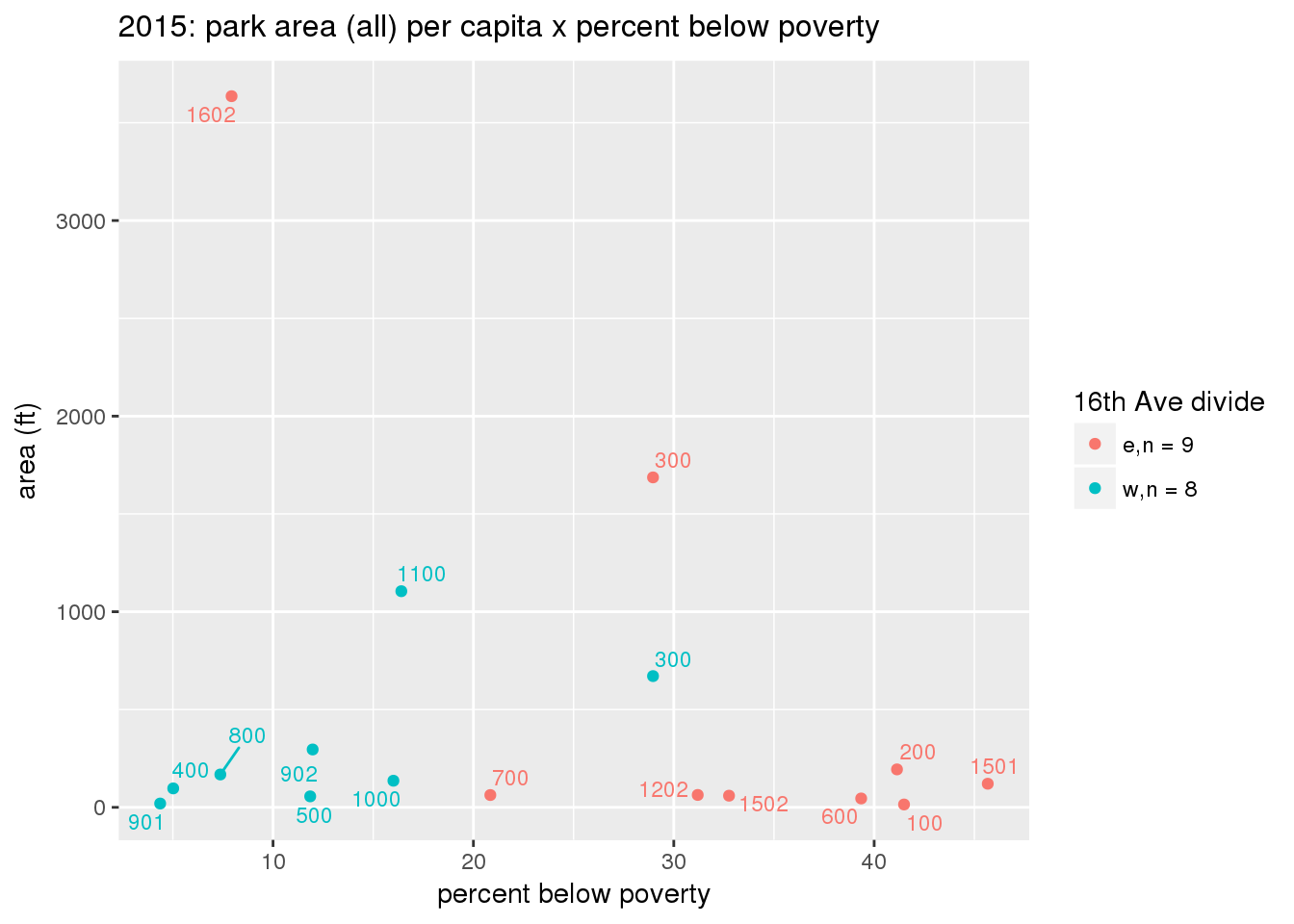
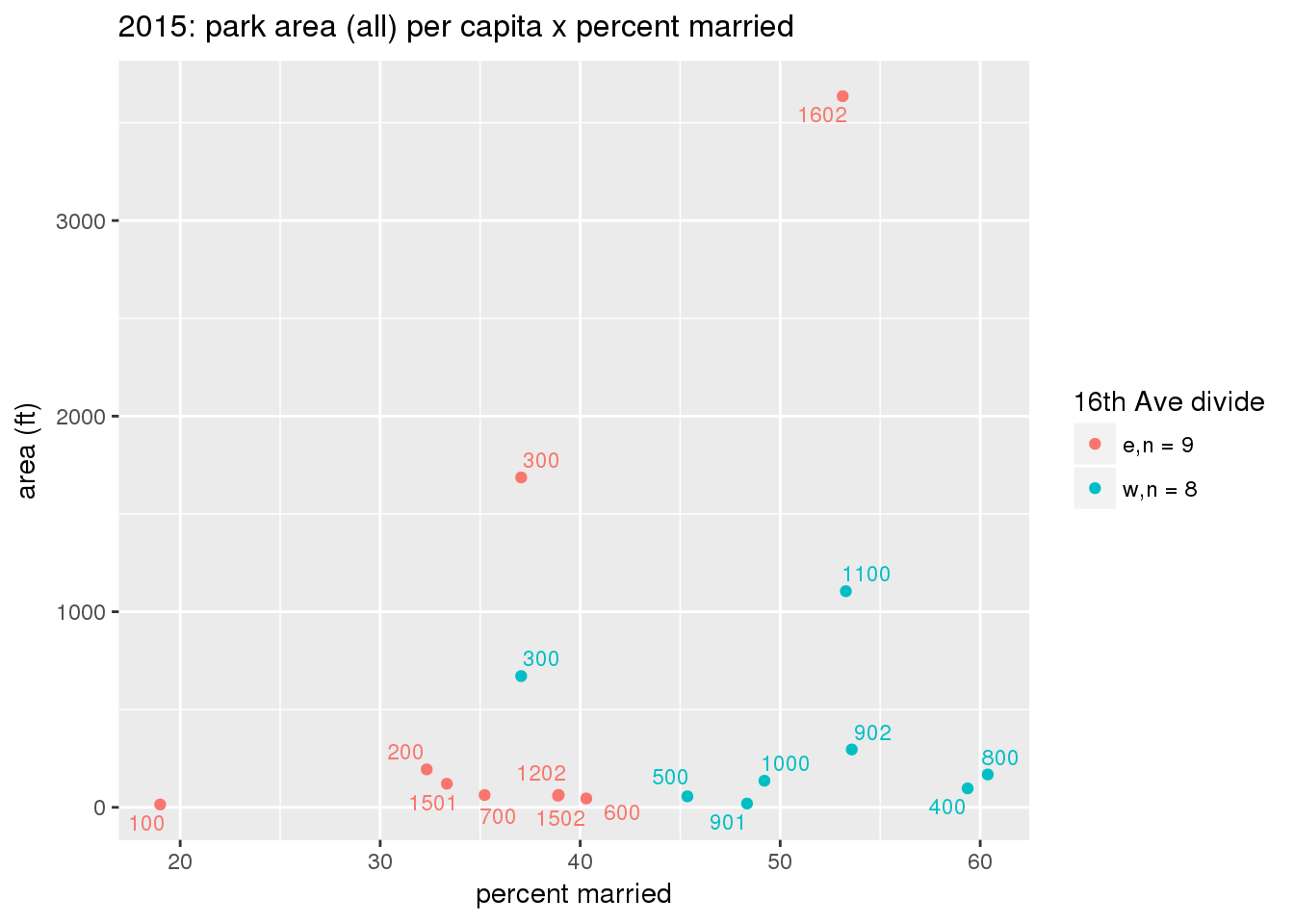
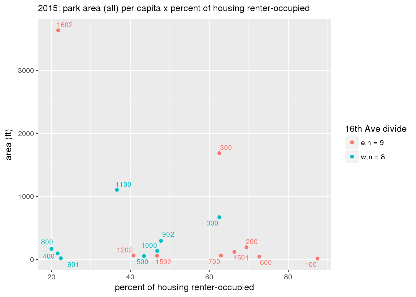
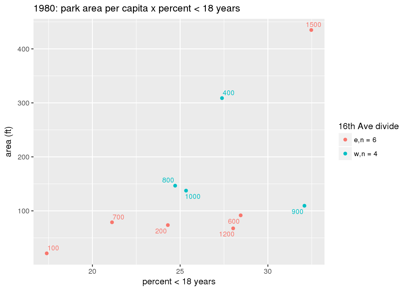
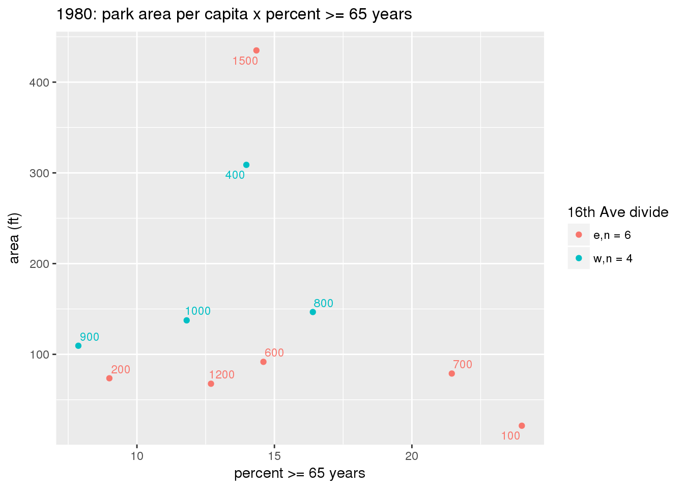
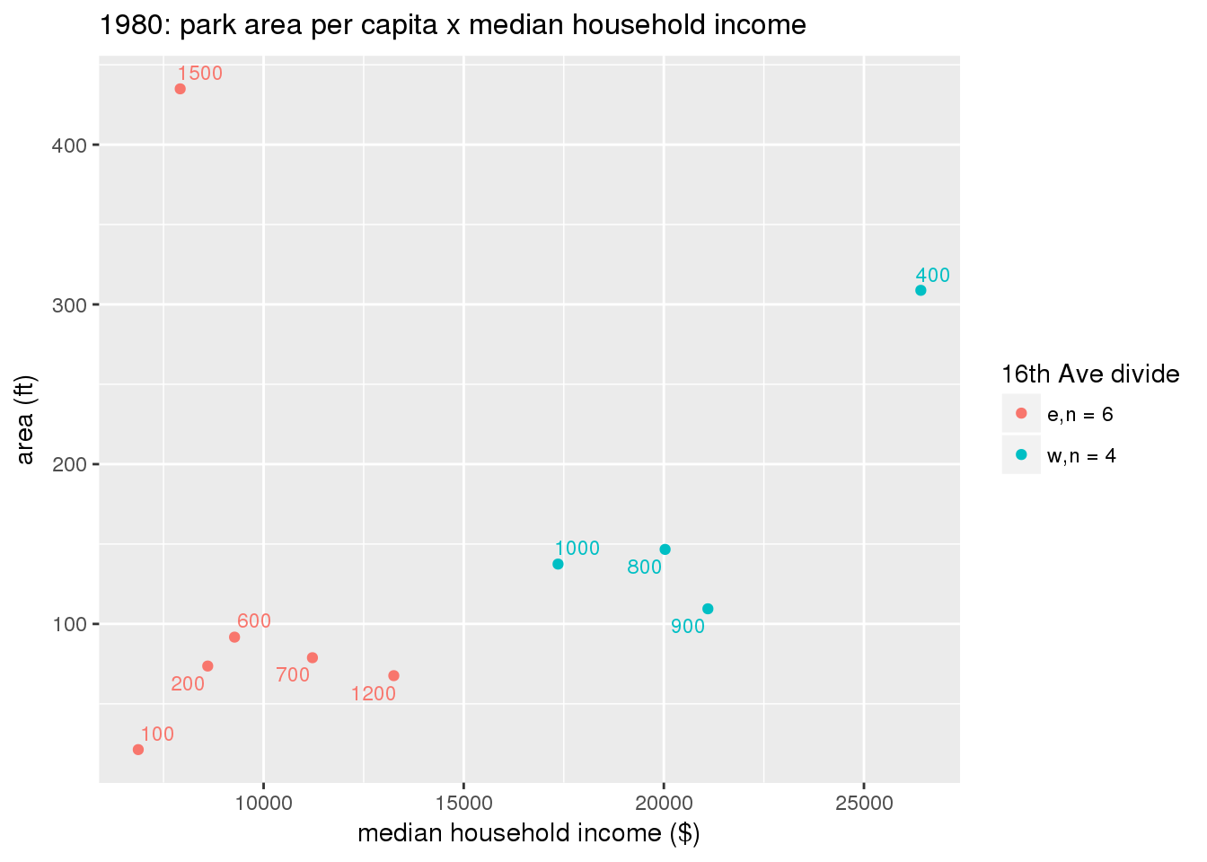
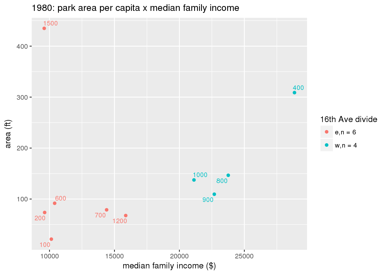
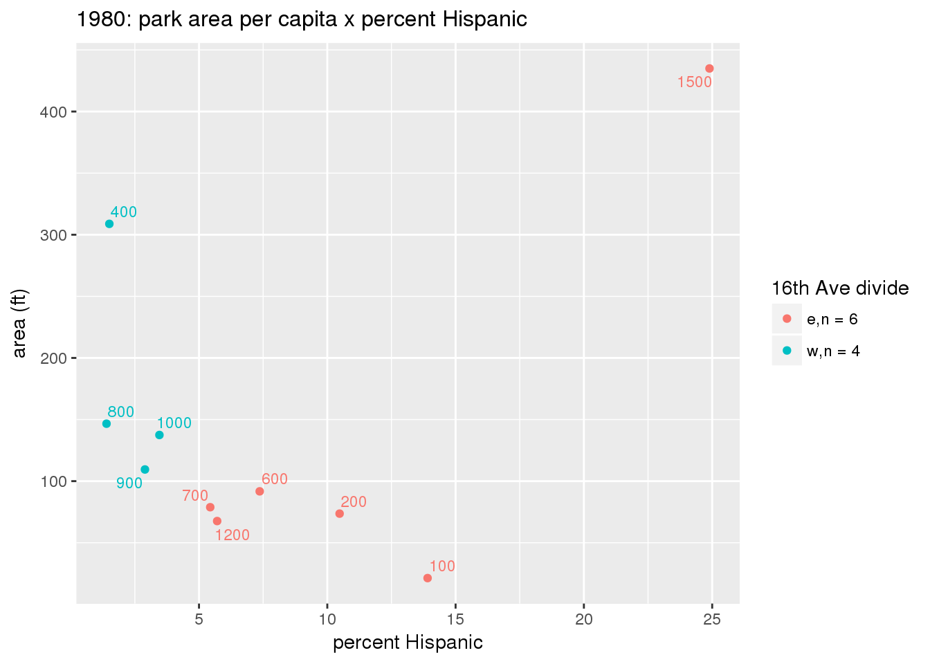
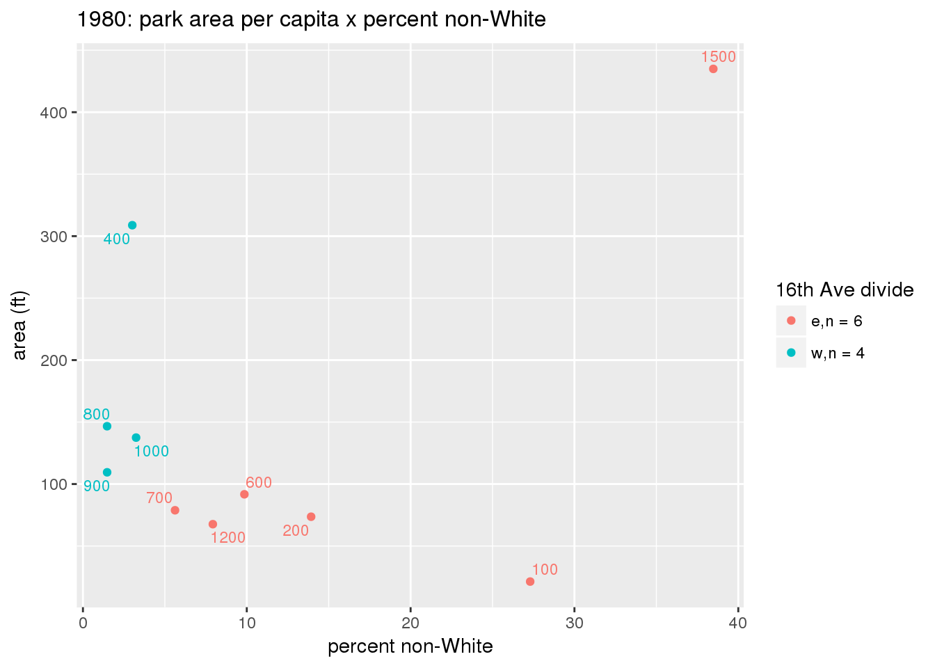
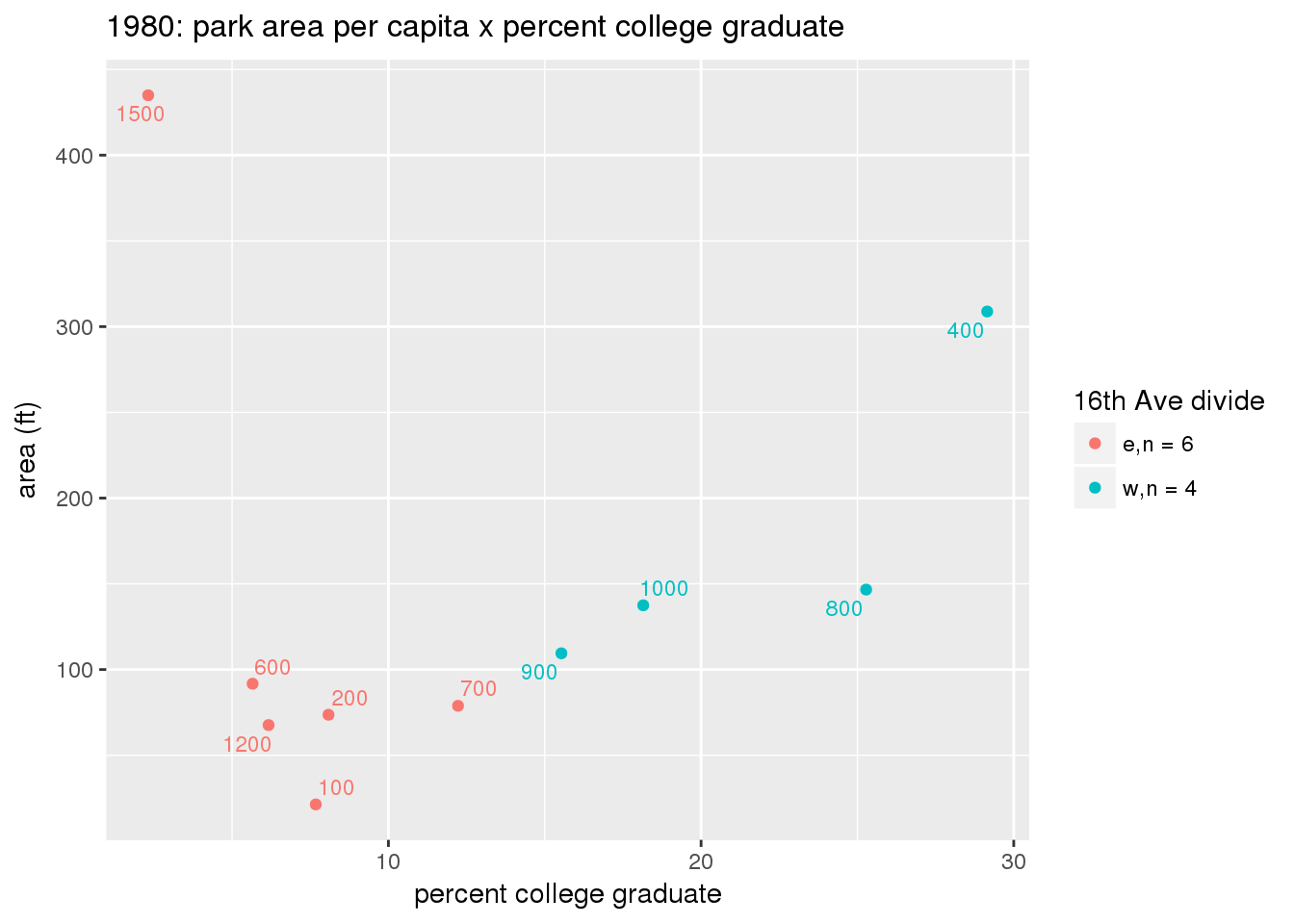
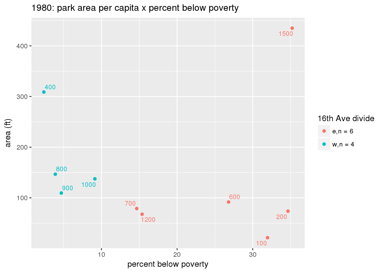
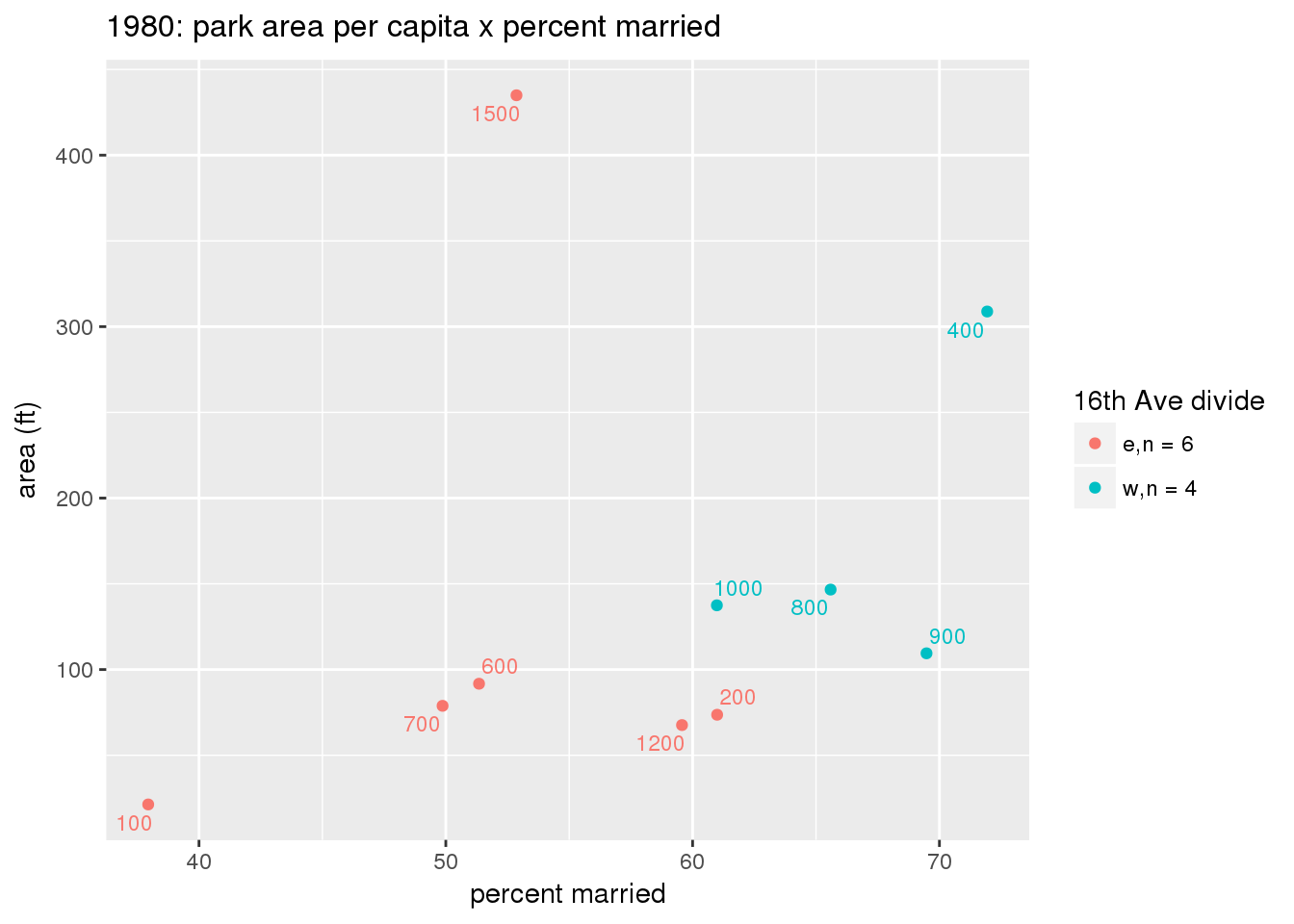
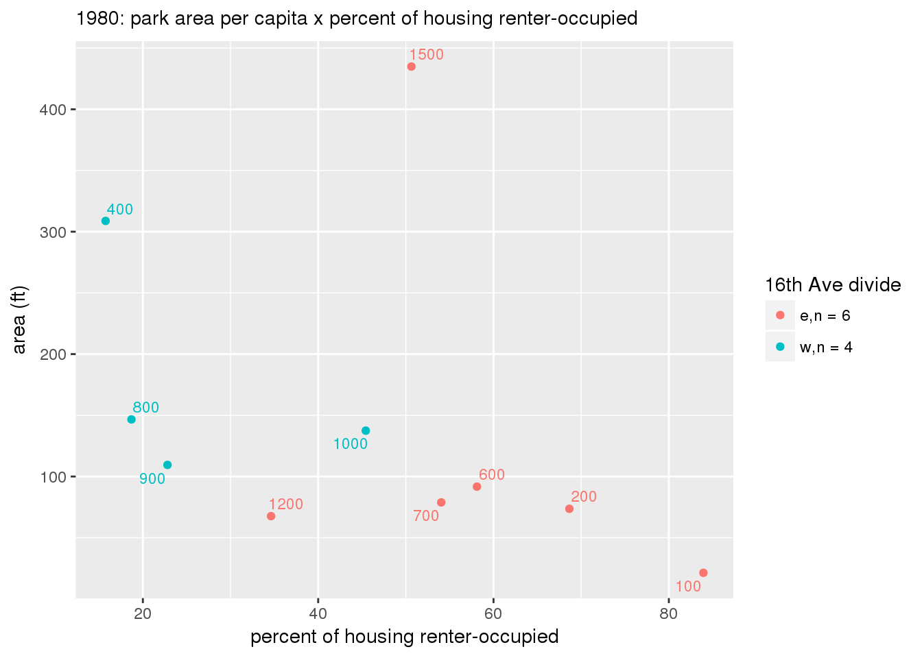
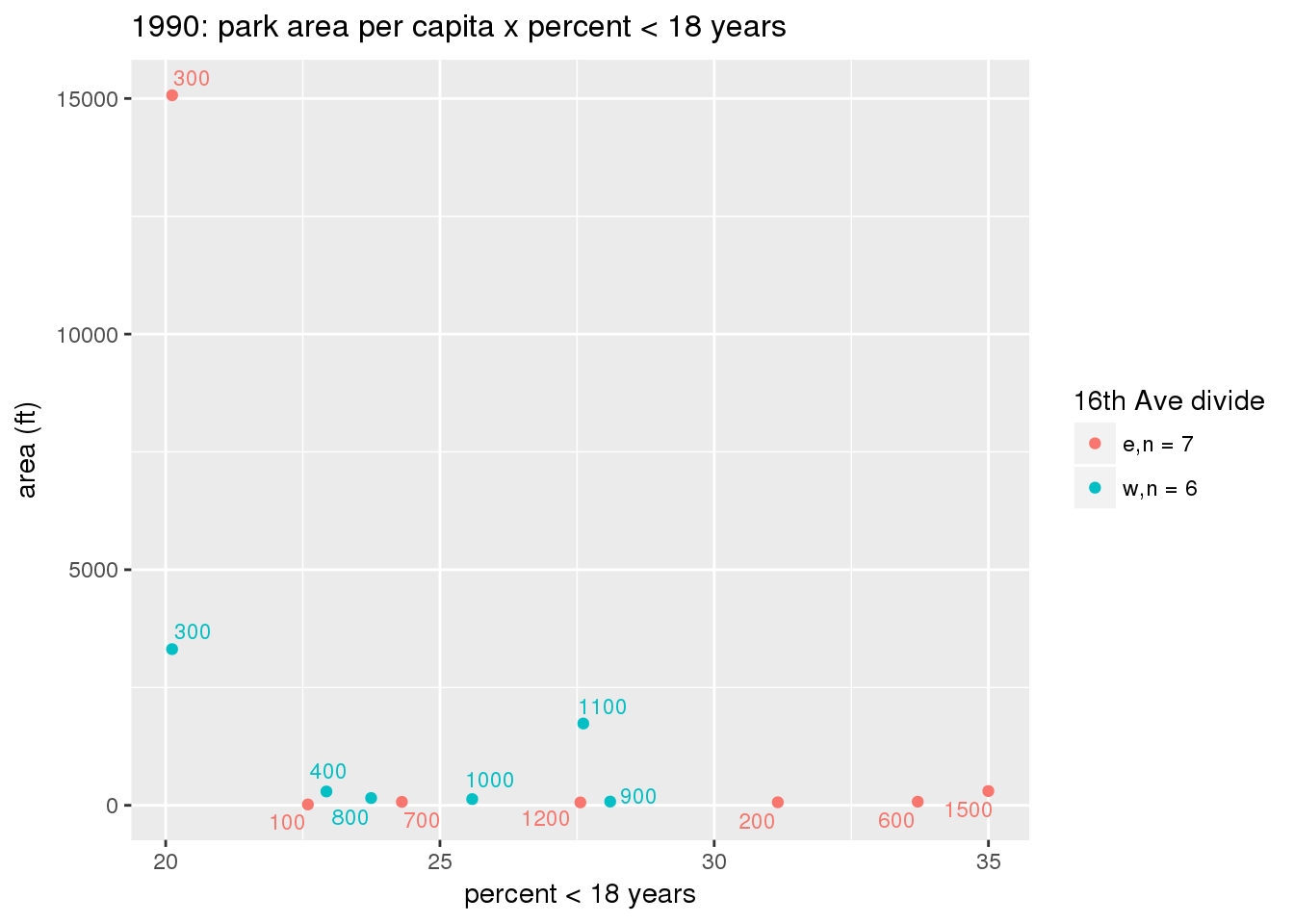
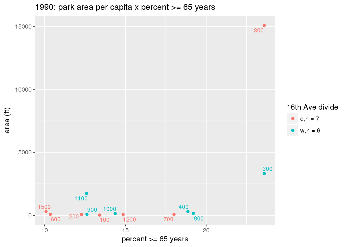
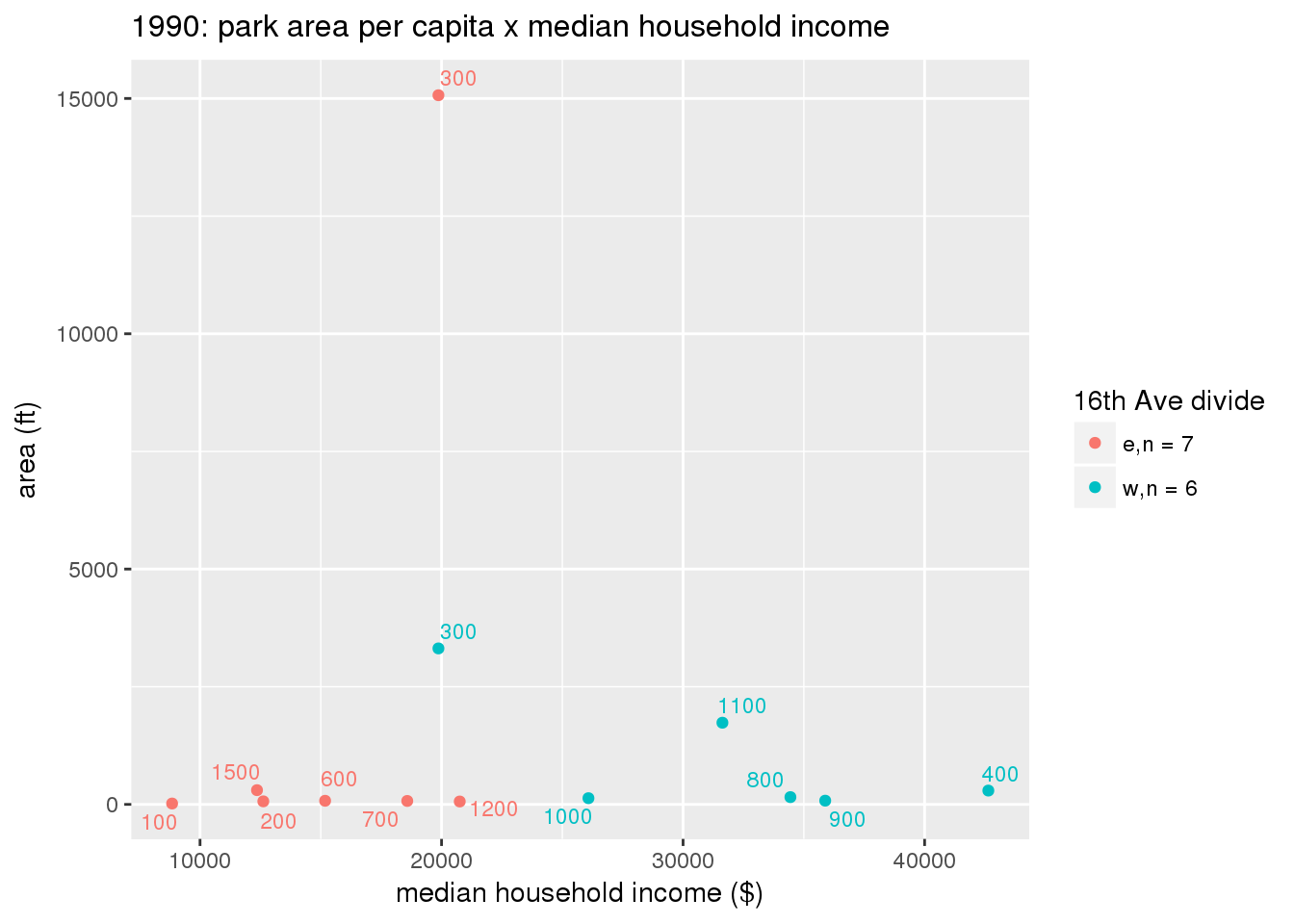
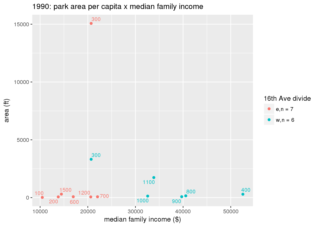
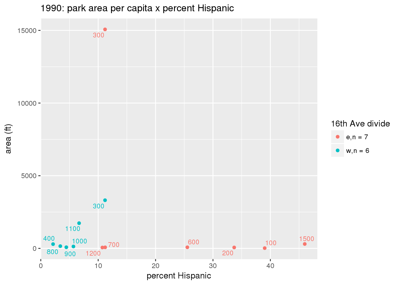
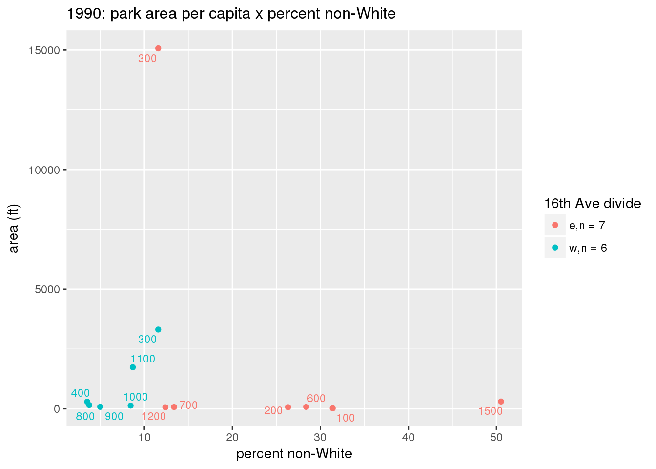
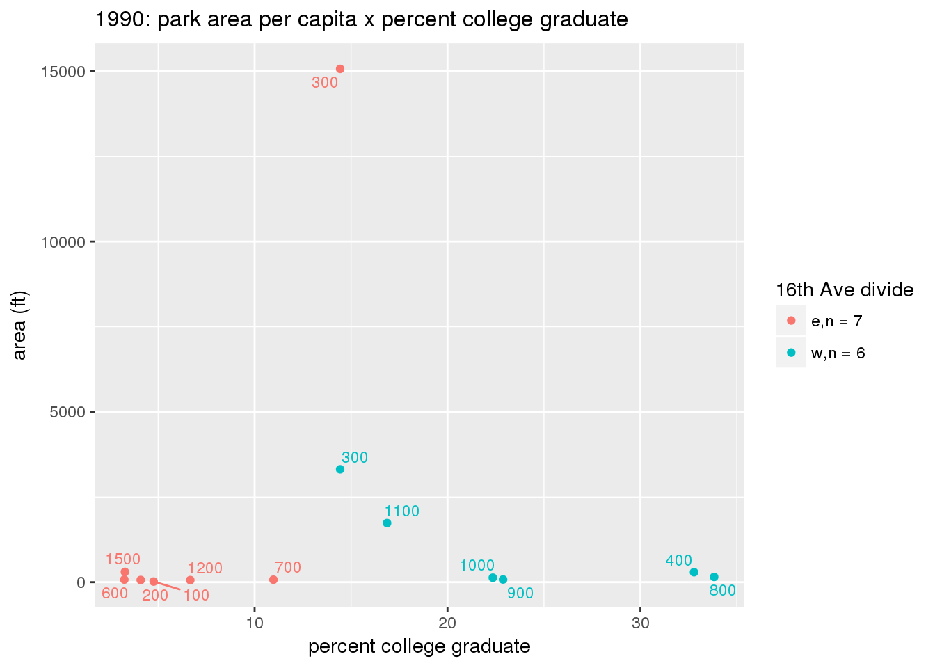
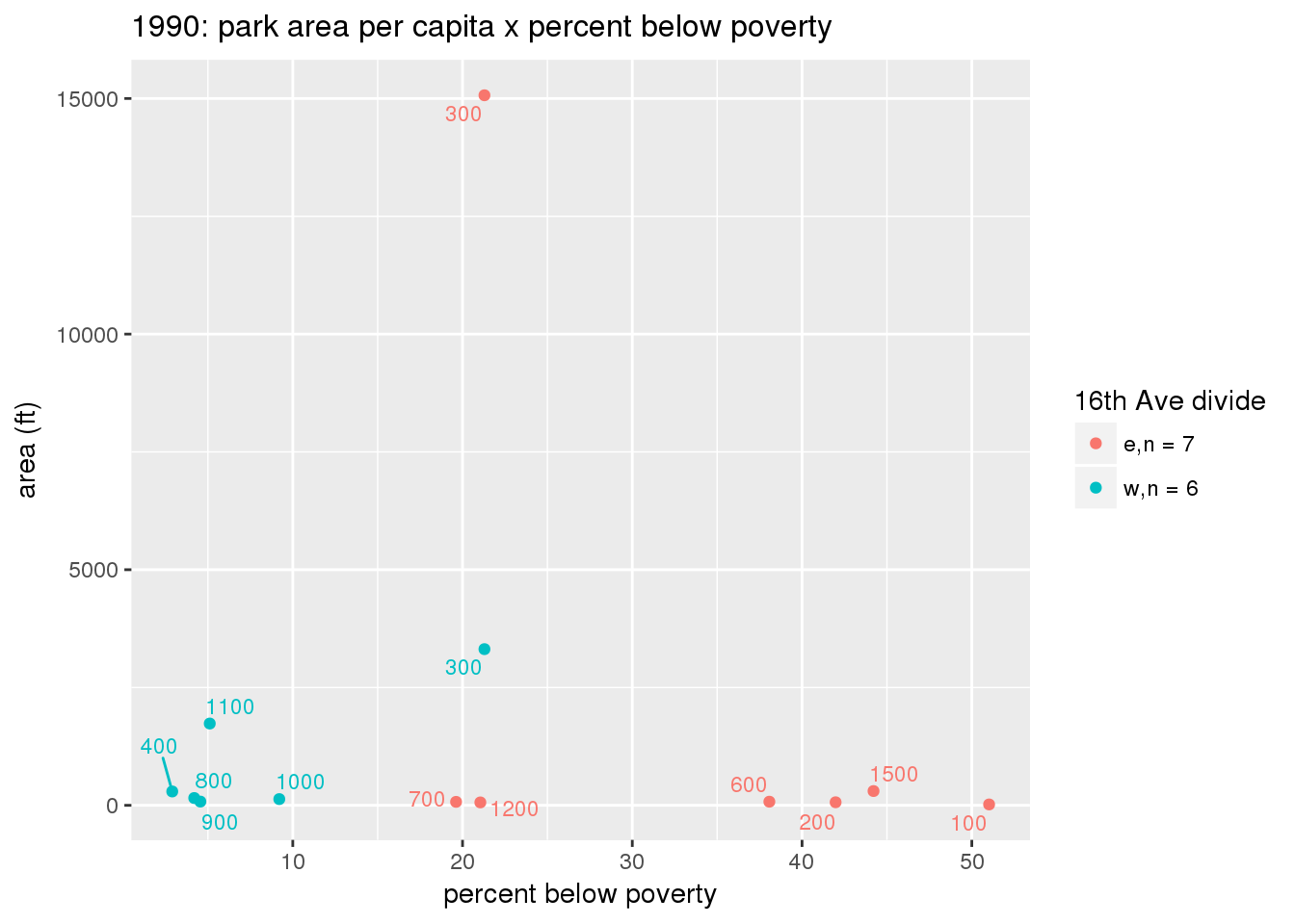
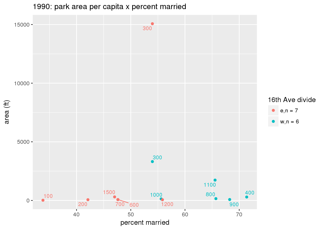
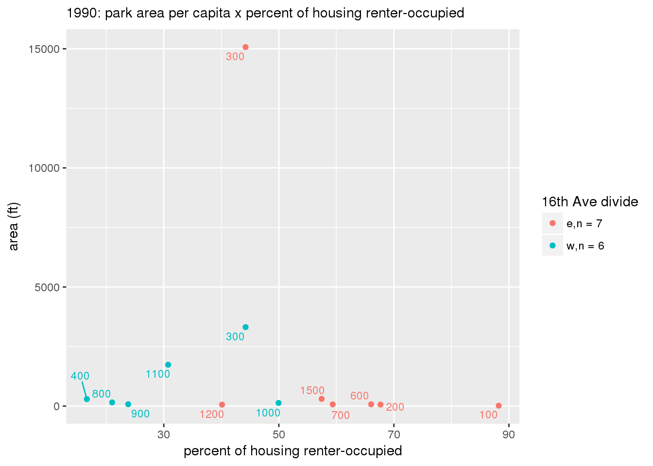
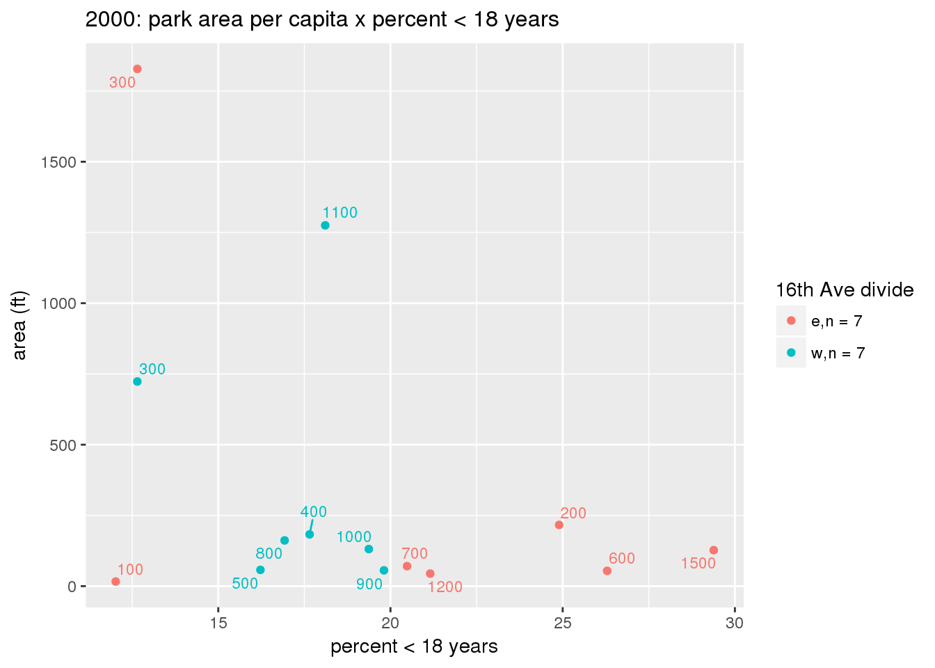
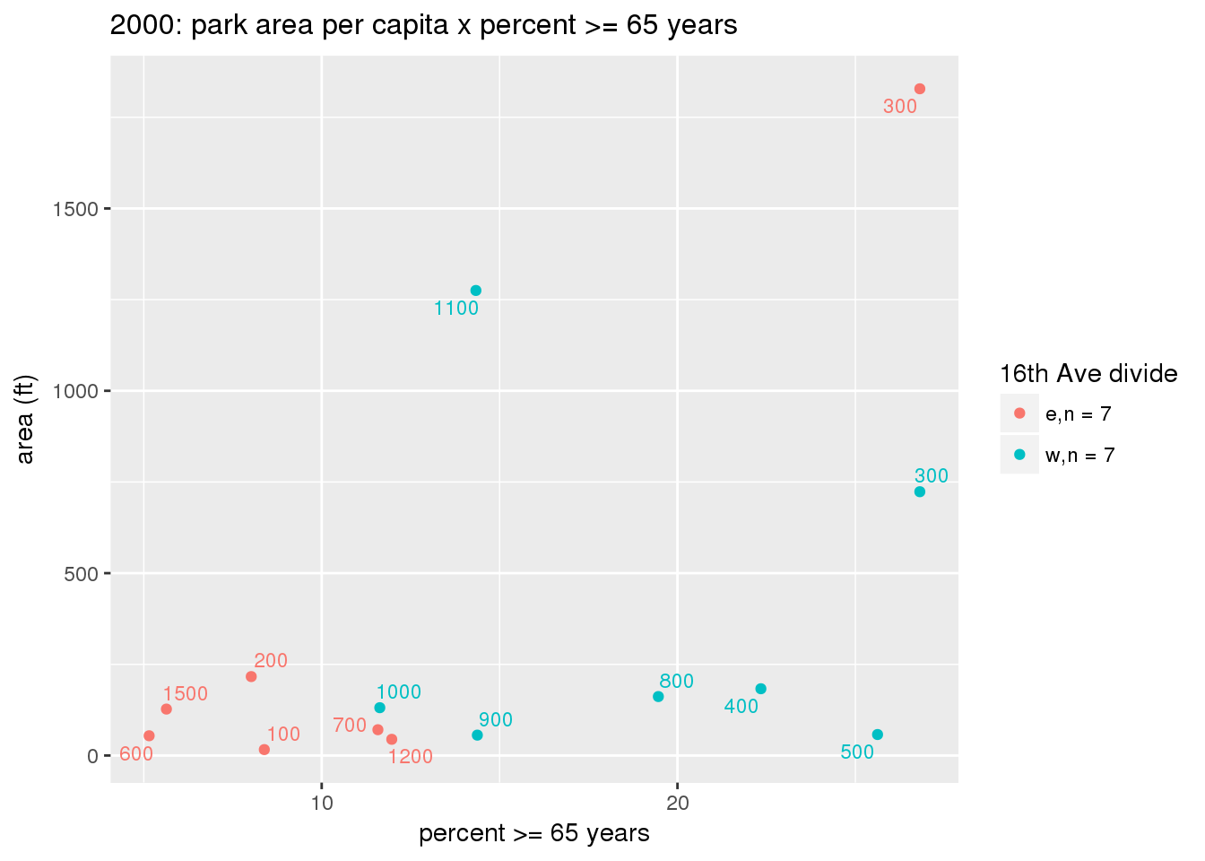
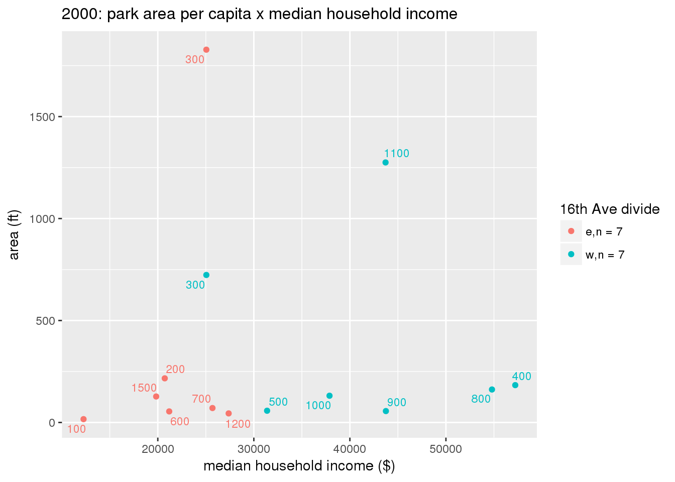
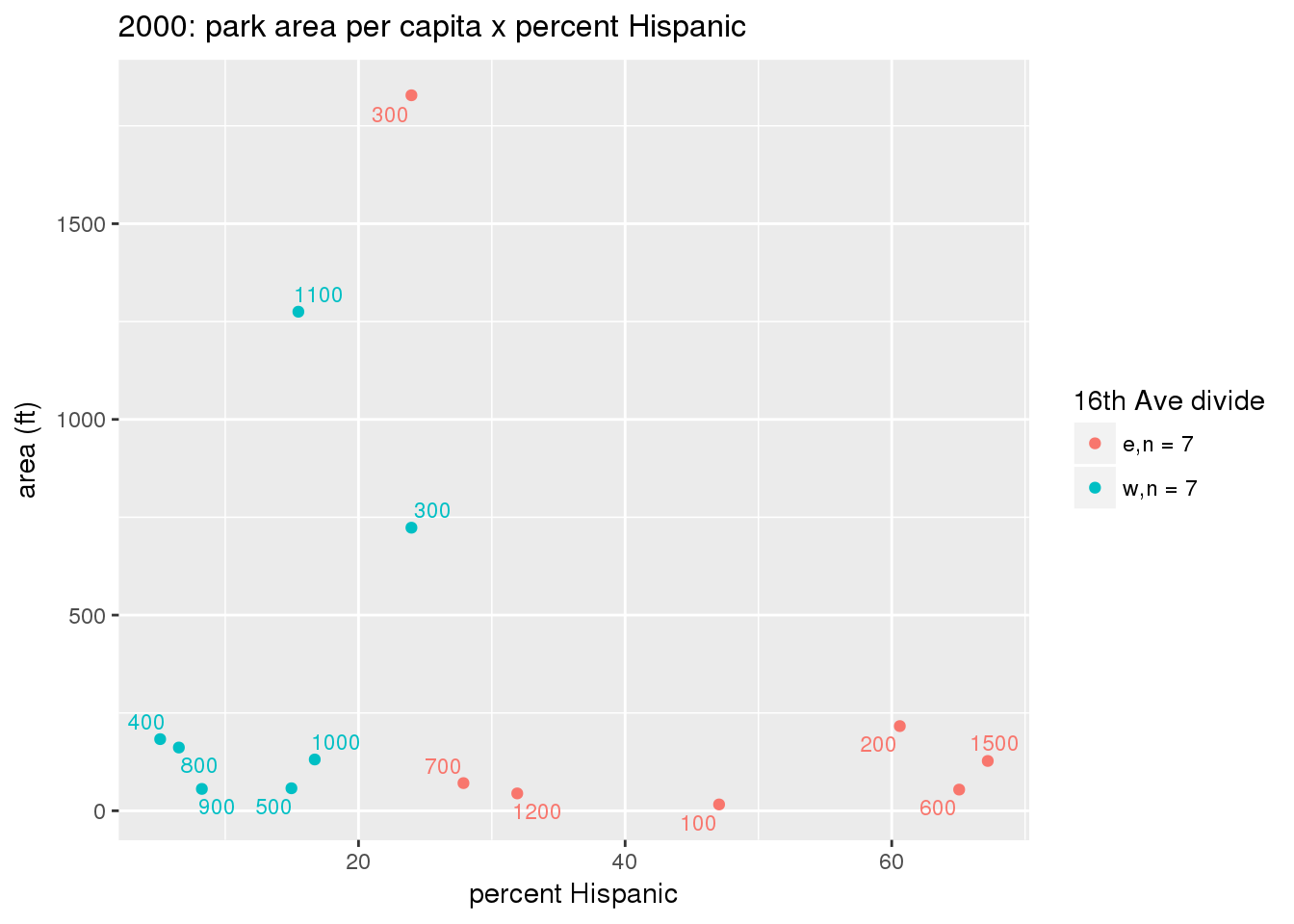
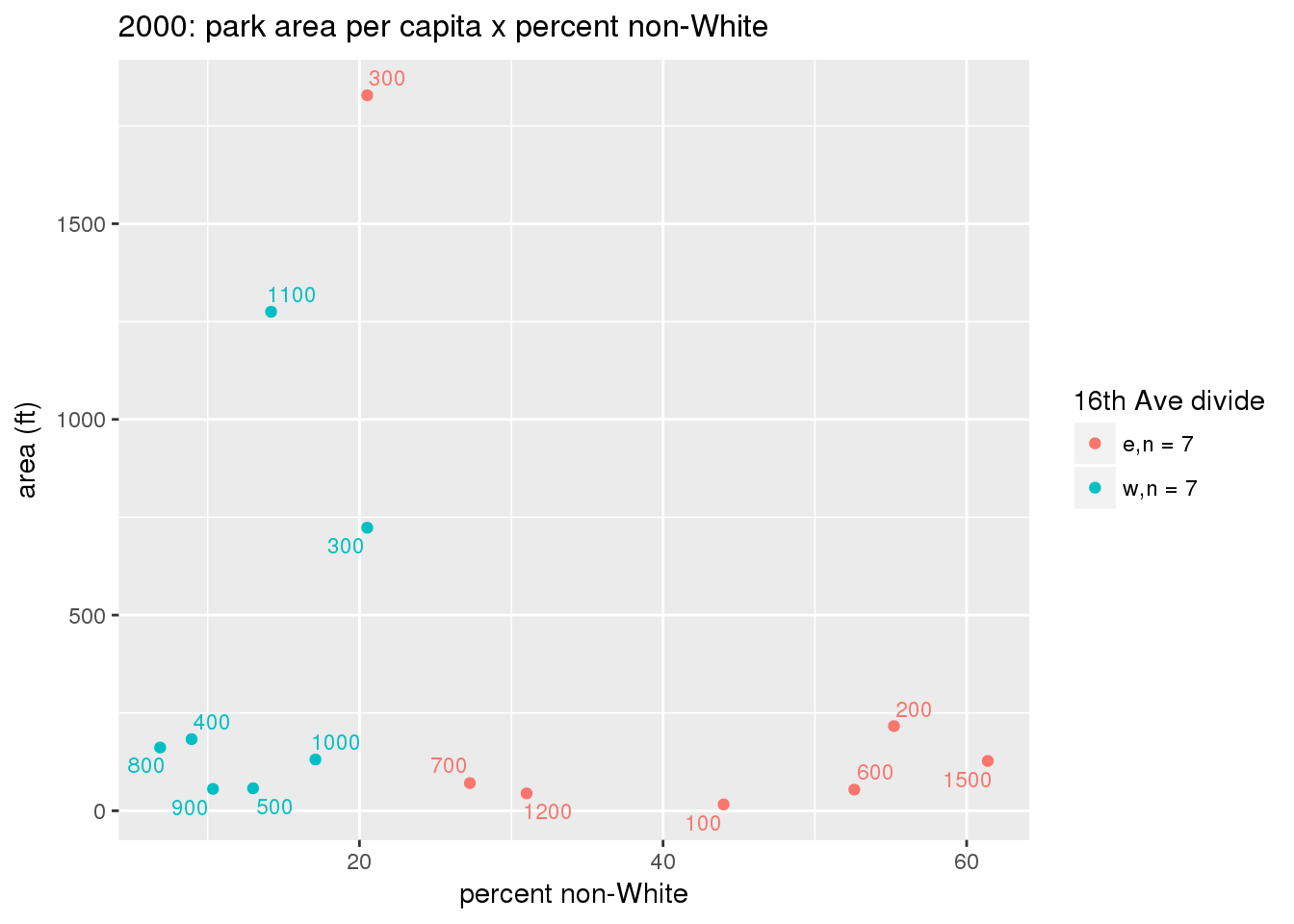
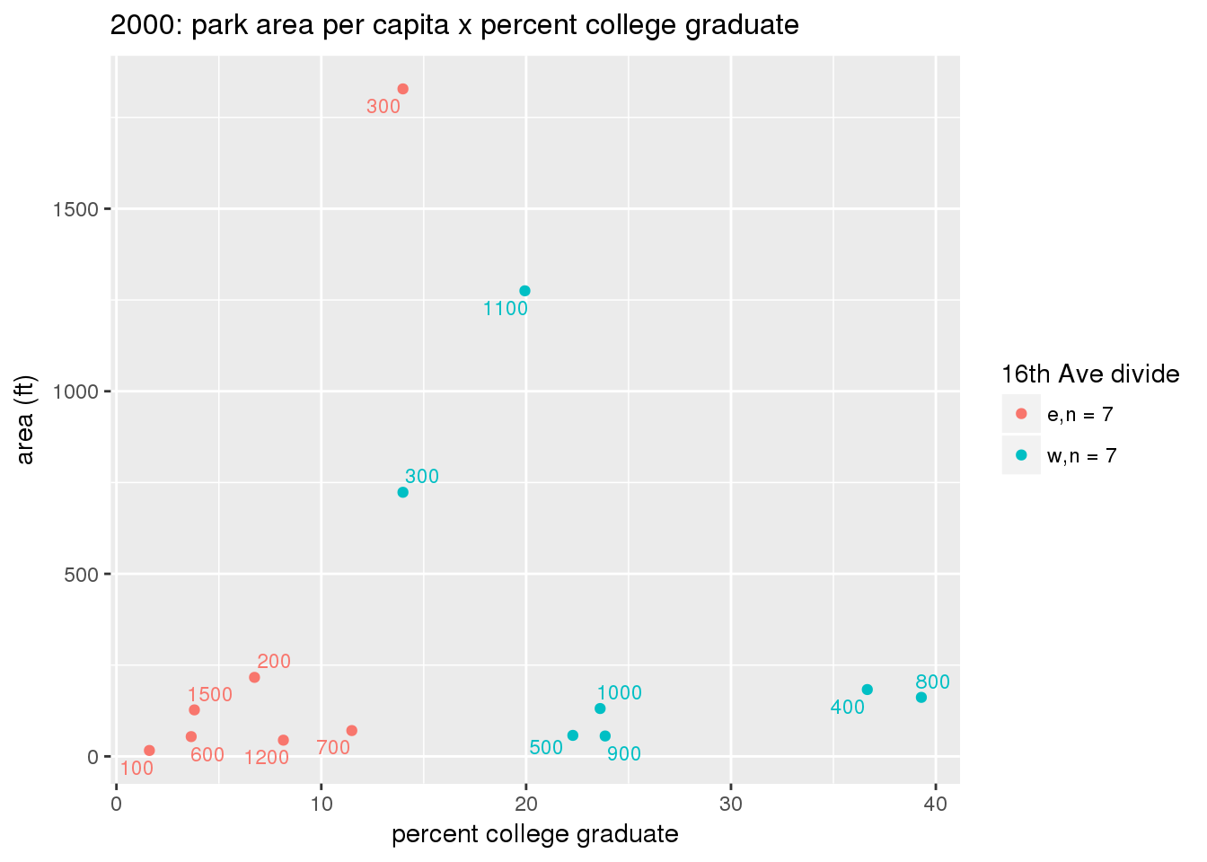
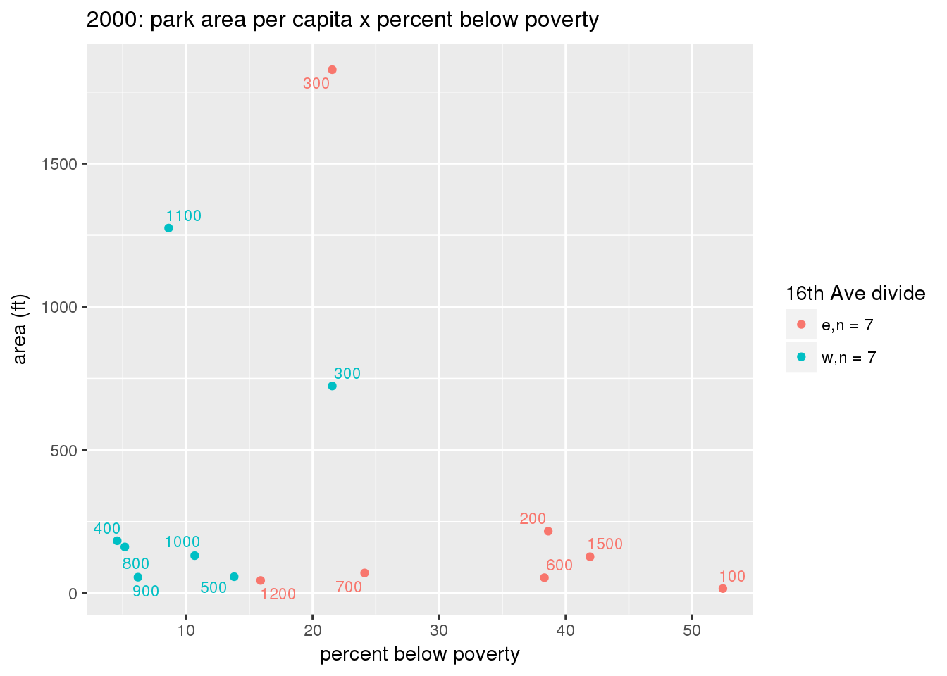
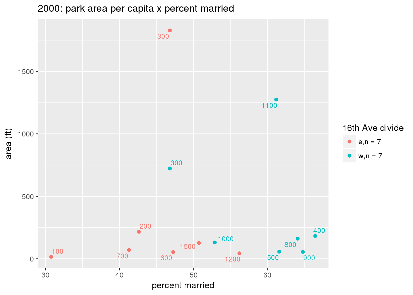
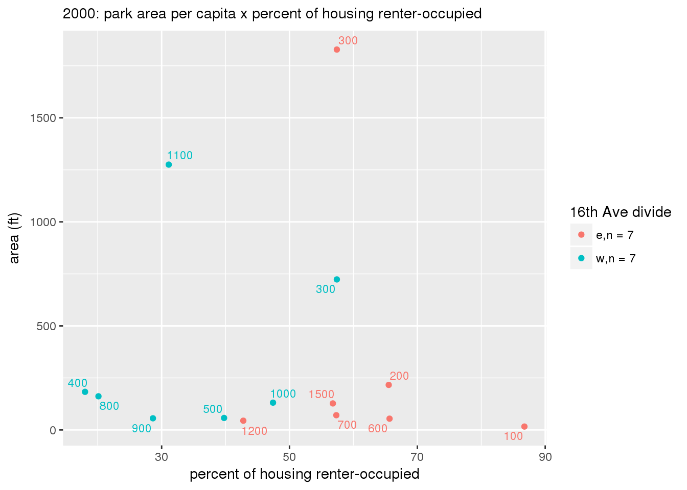
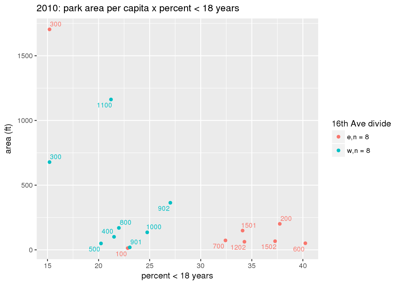
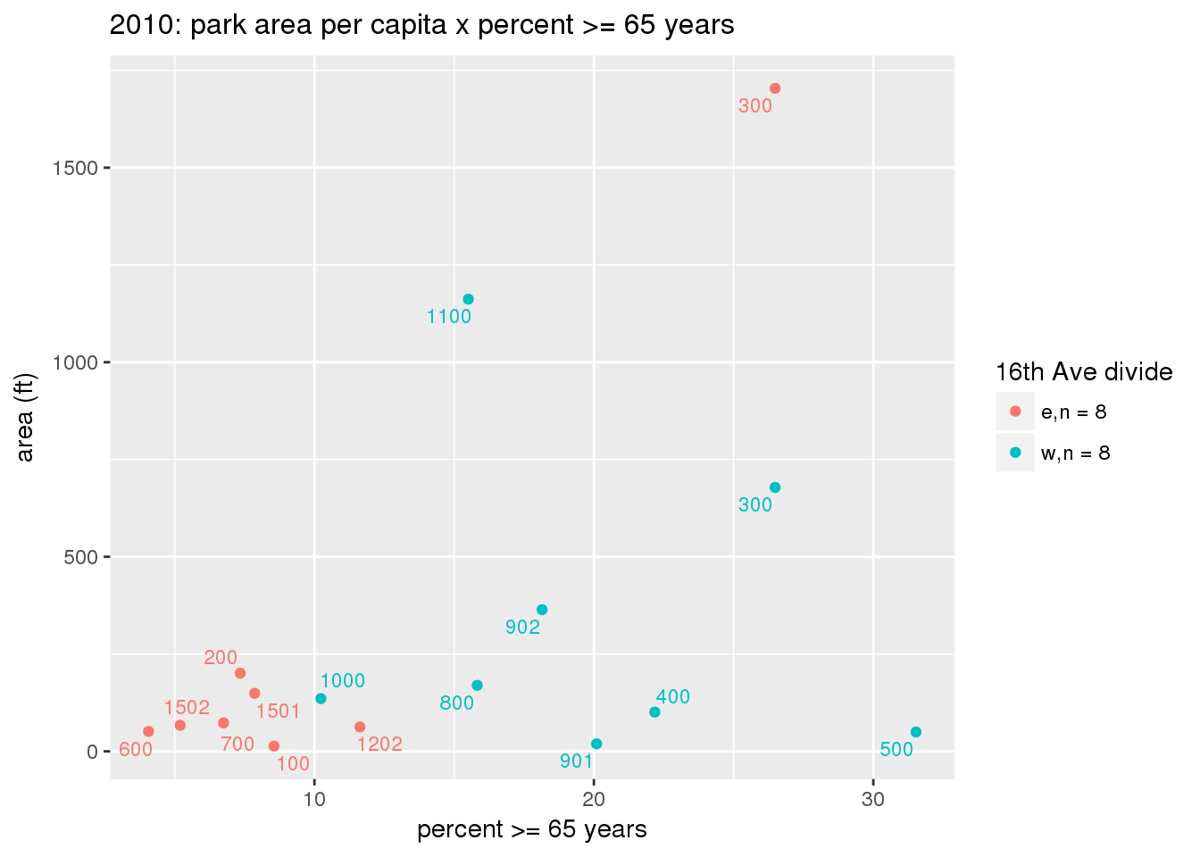
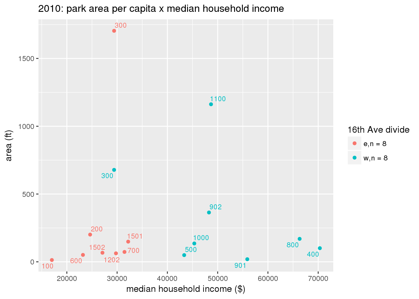
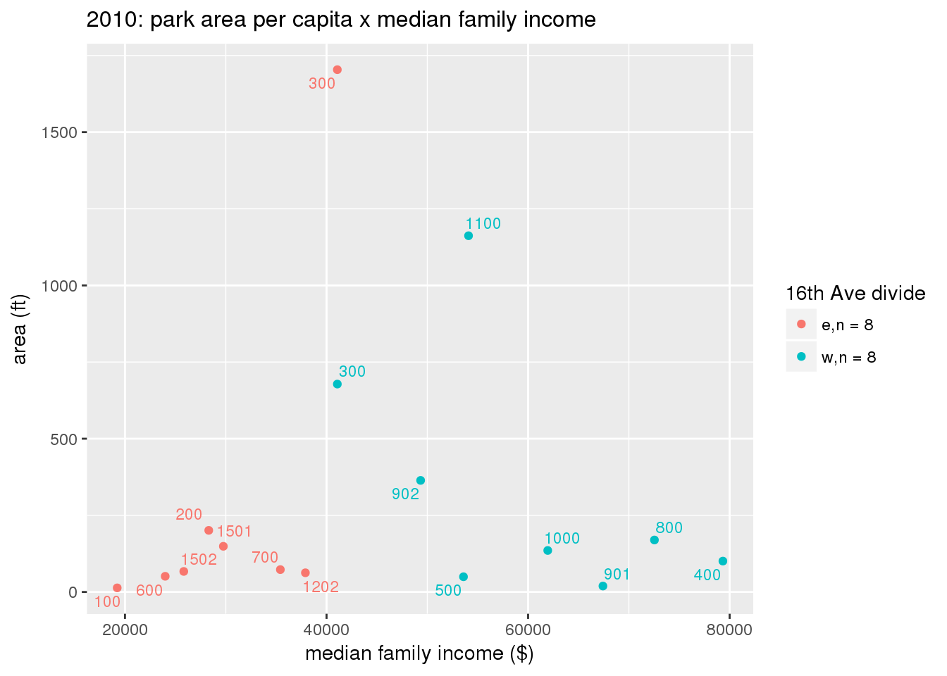
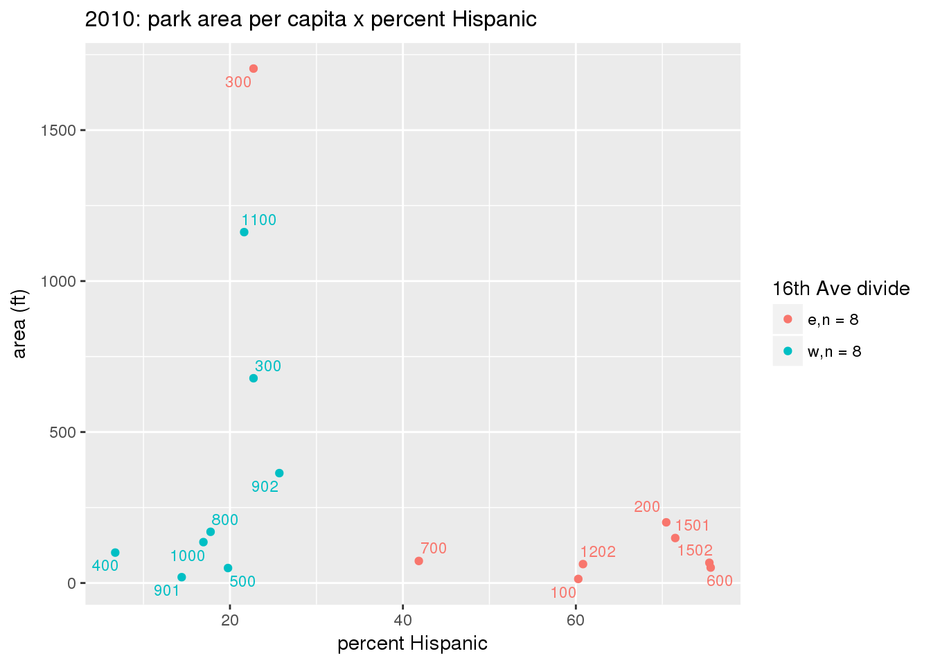
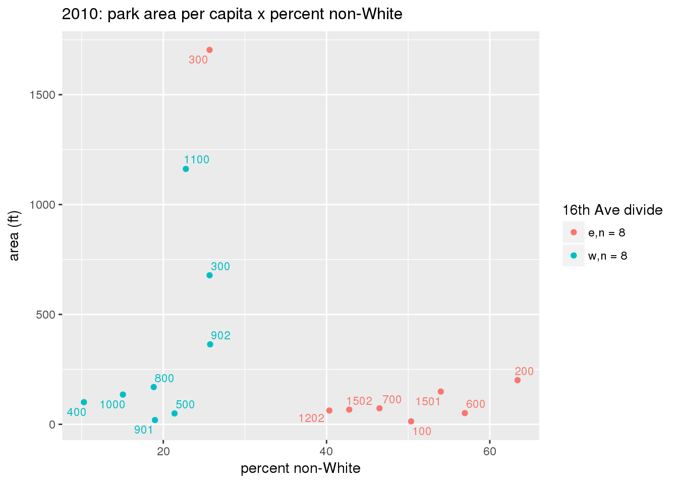
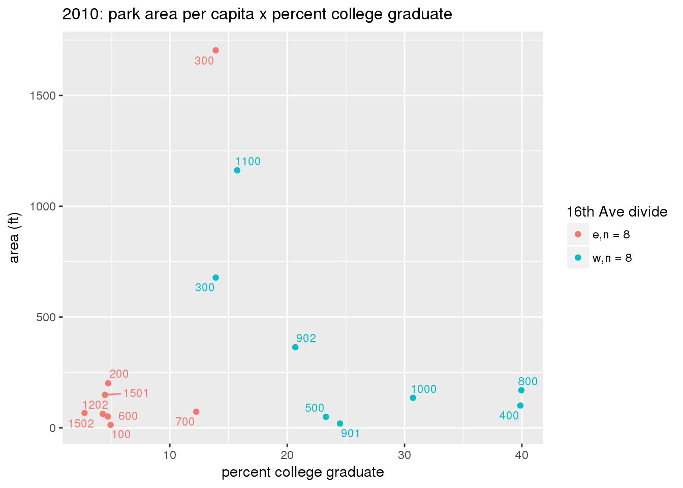
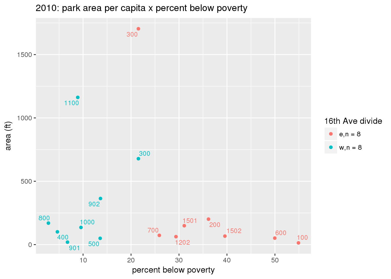
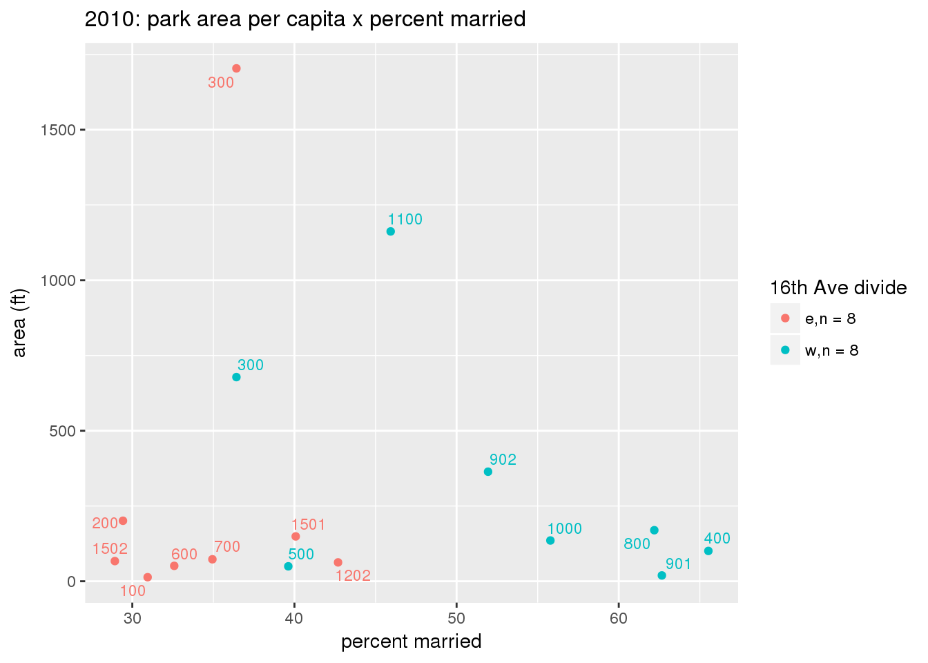
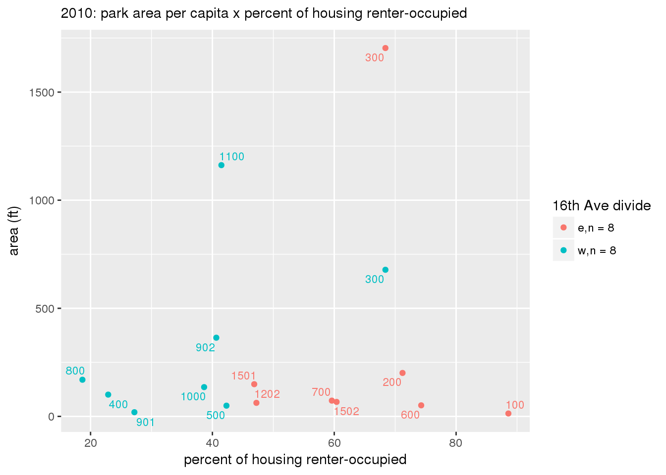
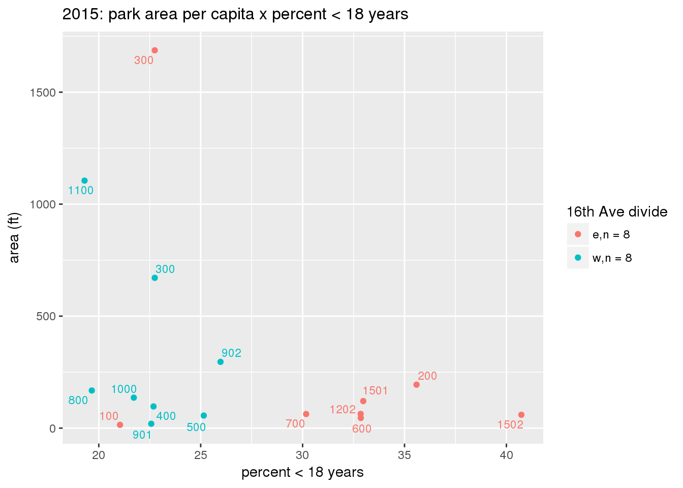
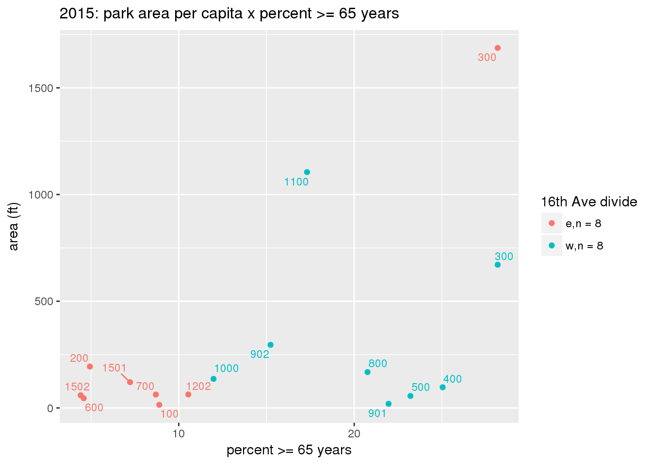
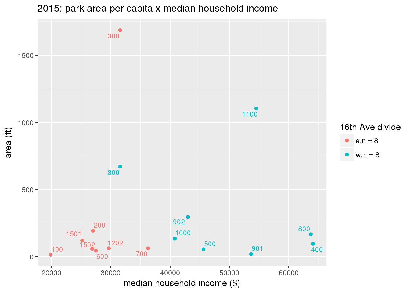
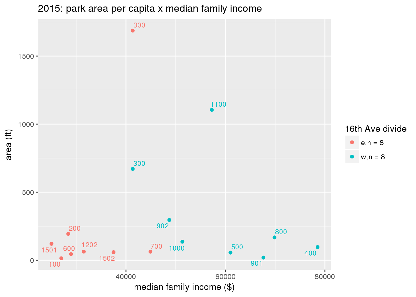
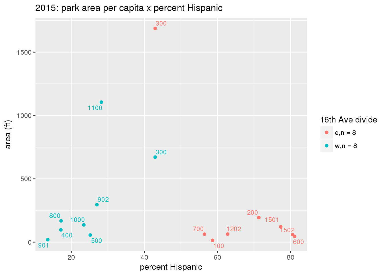
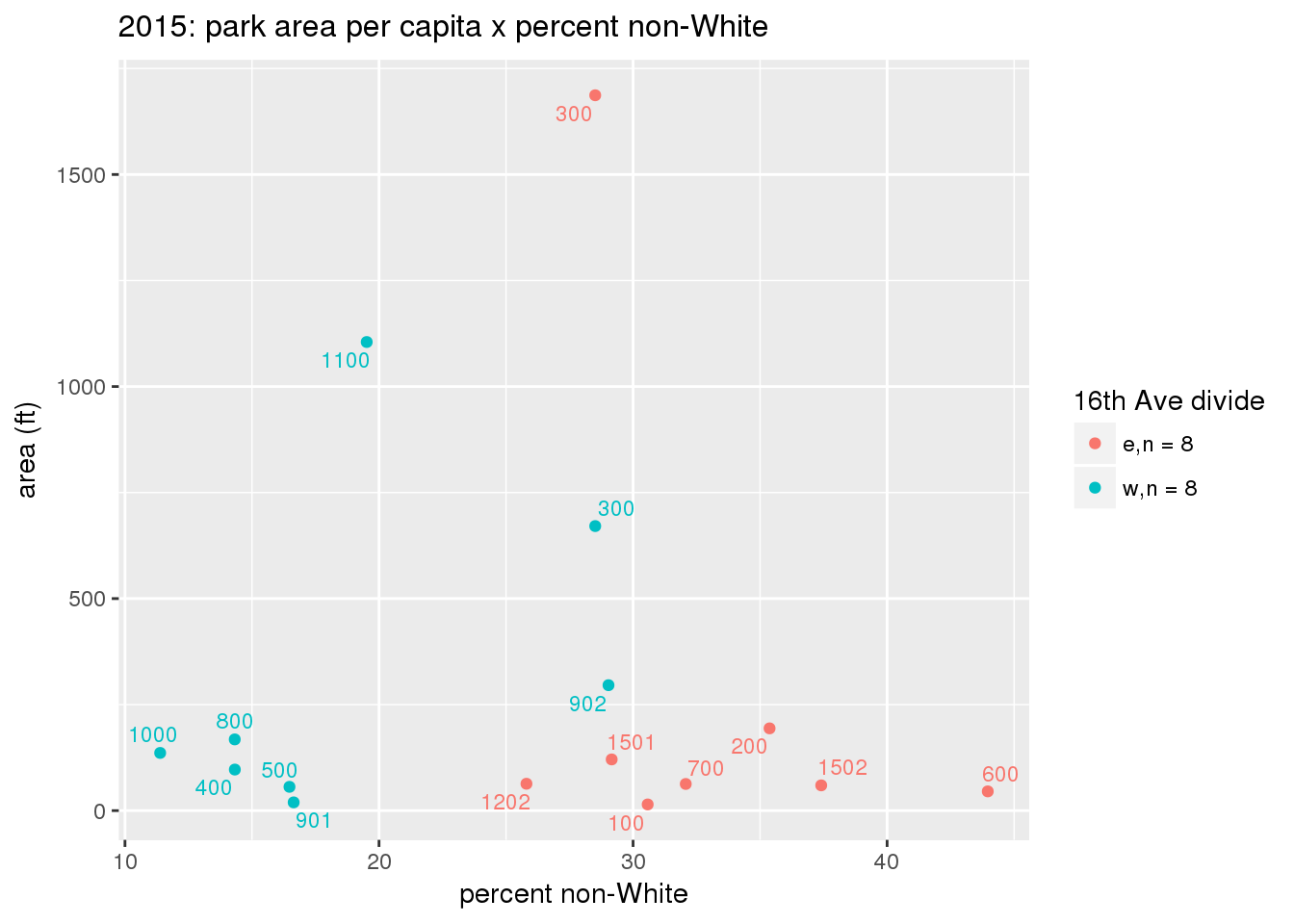
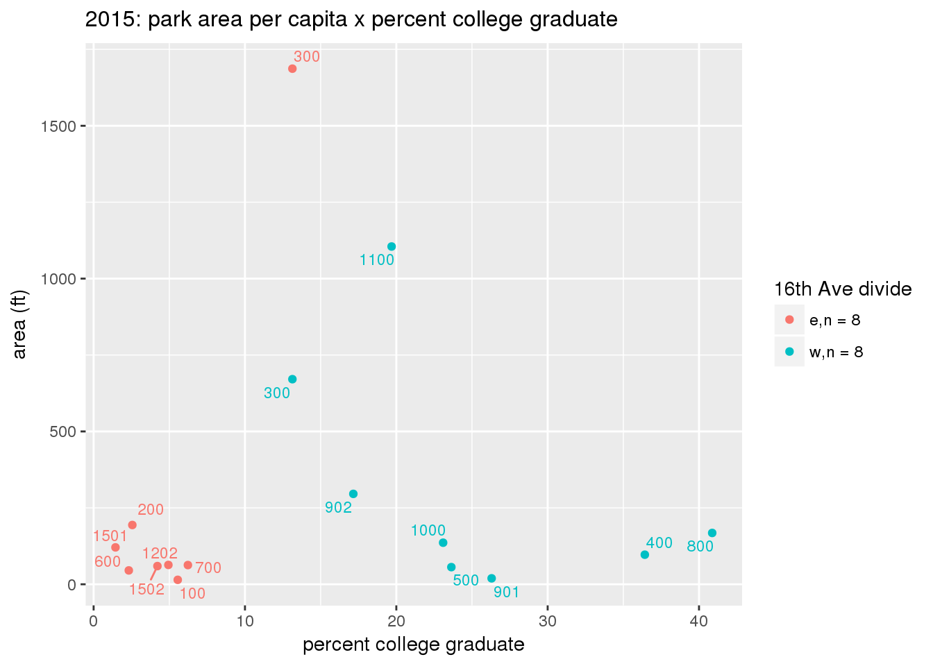
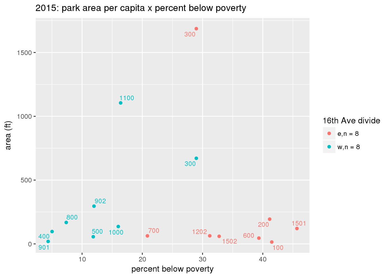
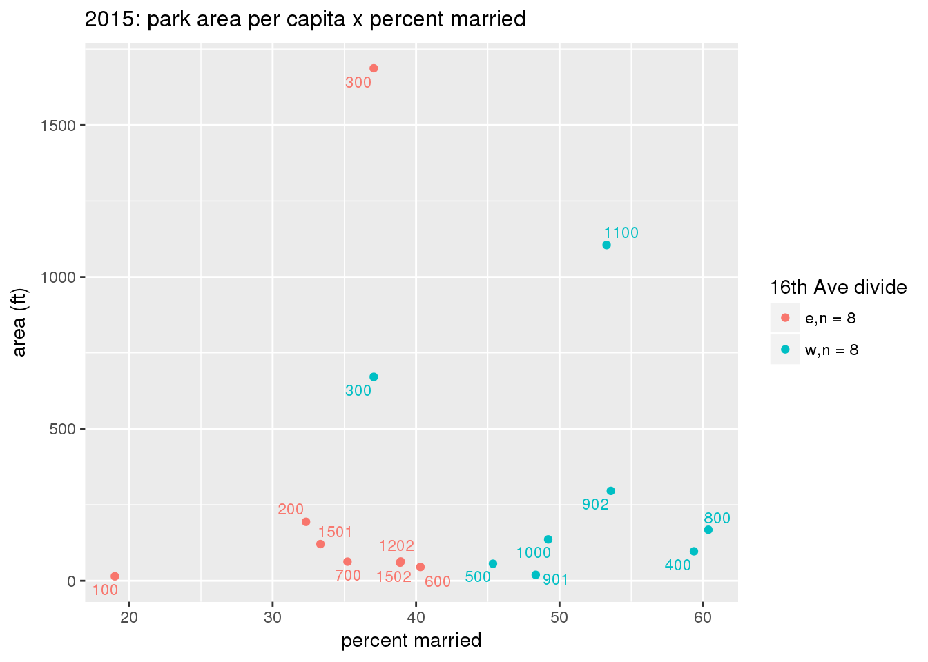
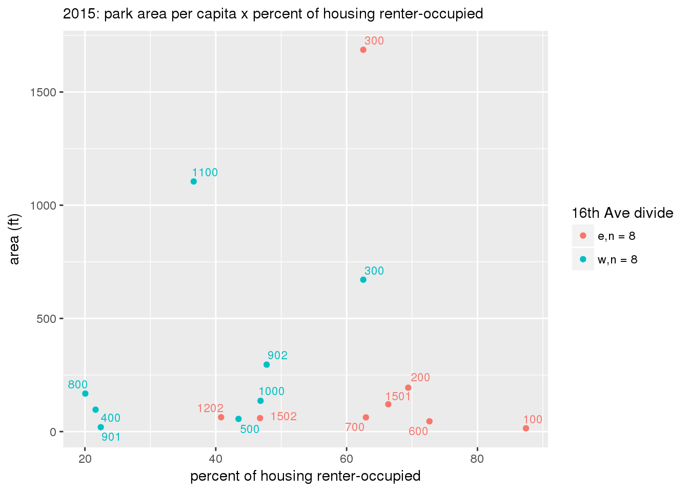
These graphs present demographic variables of interest on the X-axis and per-capita area of parks on the Y-axis, time-matched by year. Tracts were stratified by the 16th Avenue dividing line. The number of tracts per east/west group is shown in the legend.
It should be noted that for there is one census tract with a large per-capita area across each year; therefore a second set of graphs was prepared excluding the point with the greatest value in each year.
The observed stratification in the X-axis reflects general sociodemographic differences between eastern and western Yakima. The other trend seems to be that the amount of park area per capita was greater for western Yakima in 1980, but as the City grew over subsequent years, the area of park per capita became much more uniform across the 16th Avenue dividing line.
3.3.1.2.1 All tracts
3.3.1.2.1.1 Parks with no private funding
sqlbase <- "
                                                with
                                                --parks
                                                prp as (select * from yakima_equity.park_private)
                                                , p0 as (select * from yakima_equity.parksvalid where yearcreated <= xxxYEARxxx and name not in (select name from prp))
                                                , p as (select the_geom_2286, st_area(the_geom_2286) as park_area_orig from p0)
                                                --census tracts
                                                , ct as (select tract
                                                    , zone_16th
                                                    , the_geom_2286
                                                    , total_pop
                                                    , age_lt_18 / total_pop::numeric * 100 as pct_lt_18
                                                    , age_ge_65 / total_pop::numeric * 100 as pct_ge_65
                                                    , median_hh_income
                                                    , median_family_income
                                                    , eth_hispanic / total_pop::numeric * 100 as pct_hispanic
                                                    , race_nonwhite / total_pop::numeric * 100 as pct_nonwhite
                                                    , case when (edu_collgrad + edu_9th_somecoll + edu_lt_9th) = 0 then 0 else edu_collgrad::numeric / (edu_collgrad + edu_9th_somecoll + edu_lt_9th) * 100 end as pct_collgrad
                                                    , case when pov_status = 0 then 0 else pov_below_100pct / pov_status::numeric * 100 end as pct_below_poverty
                                                    , case when married + unmarried = 0 then 0 else married / (married + unmarried)::numeric * 100 end as pct_married
                                                    , case when housingunits_renter + housingunits_owner = 0 then 0 else housingunits_renter / (housingunits_renter + housingunits_owner)::numeric * 100 end as pct_renter
                                                    from yakima_equity.tract_xxxYEARxxx)
                                                --intersection
                                                , i as (select tract, zone_16th, park_area_orig, st_intersection(p.the_geom_2286, ct.the_geom_2286) as geom_clip from p, ct where st_intersects(p.the_geom_2286, ct.the_geom_2286))
                                                --area
                                                , a as (select tract, sum(st_area(geom_clip)) as area_ft from i group by tract order by tract)
                                                --join
                                                , j as (select tract, coalesce(area_ft, 0) as area_ft
                                                    , zone_16th
                                                    , total_pop
                                                    , coalesce(area_ft / total_pop, 0) as sqft_per_person
                                                    , pct_lt_18
                                                    , pct_ge_65
                                                    , median_hh_income
                                                    , median_family_income
                                                    , pct_hispanic
                                                    , pct_nonwhite
                                                    , pct_nonwhite
                                                    , pct_collgrad
                                                    , pct_below_poverty
                                                    , pct_married
                                                    , pct_renter
                                                from a full join ct using(tract) order by tract)
                                                select * from j where area_ft > 0;"

                                                #for(y in c(2010)){
                                                for(y in c(1980, 1990, 2000, 2010, 2015)){
                                                #message(y)
                                                    sqly <- gsub("xxxYEARxxx", y, sqlbase)

                                                    assign("sqly", sqly, envir = .GlobalEnv)

                                                    x <- dbGetQuery(conn = dbconn, statement = sqly)

                                                    xvars <- list(
                                                        c('pct_lt_18', 'percent < 18 years'),
                                                        c('pct_ge_65', 'percent >= 65 years'),
                                                        c('median_hh_income', 'median household income'),
                                                        c('median_family_income', 'median family income'),
                                                        c('pct_hispanic', 'percent Hispanic'),
                                                        c('pct_nonwhite', 'percent non-White'),
                                                        c('pct_collgrad', 'percent college graduate'),
                                                        c('pct_below_poverty', 'percent below poverty'),
                                                        c('pct_married', 'percent married'),
                                                        c('pct_renter', 'percent of housing renter-occupied'))


                                                    for(i in xvars){
                                                    #message(i)
                                                    mytitle <- sprintf("%s: park (no private) area per capita x %s", y, i[2])
                                                    xlab <- gsub("income", "income ($)", gsub("pct_", "percent", i[2]))
                                                    ylab <- "area (ft)"
                                                    g <- corplotgg_fill(dat = x, xvar = i[1], yvar = 'sqft_per_person', fillvar = "zone_16th", mytitle = mytitle, xlab = xlab, ylab = ylab, legend_title = "16th Ave divide")
                                                    print(g)
                                                    ggsave(filename = file.path(imagedir, sprintf("%s_park_noprivate_%s.png", y, i[2])), width = ggsavewidth, height = ggsaveheight)
                                                    }
                                                }


3.3.1.2.1.2 All parks
sqlbase <- "
                                                with
                                                --parks
                                                prp as (select * from yakima_equity.park_private)
                                                , p0 as (select * from yakima_equity.parksvalid where yearcreated <= xxxYEARxxx)
                                                , p as (select the_geom_2286, st_area(the_geom_2286) as park_area_orig from p0)
                                                --census tracts
                                                , ct as (select tract
                                                    , zone_16th
                                                    , the_geom_2286
                                                    , total_pop
                                                    , age_lt_18 / total_pop::numeric * 100 as pct_lt_18
                                                    , age_ge_65 / total_pop::numeric * 100 as pct_ge_65
                                                    , median_hh_income
                                                    , median_family_income
                                                    , eth_hispanic / total_pop::numeric * 100 as pct_hispanic
                                                    , race_nonwhite / total_pop::numeric * 100 as pct_nonwhite
                                                    , case when (edu_collgrad + edu_9th_somecoll + edu_lt_9th) = 0 then 0 else edu_collgrad::numeric / (edu_collgrad + edu_9th_somecoll + edu_lt_9th) * 100 end as pct_collgrad
                                                    , case when pov_status = 0 then 0 else pov_below_100pct / pov_status::numeric * 100 end as pct_below_poverty
                                                    , case when married + unmarried = 0 then 0 else married / (married + unmarried)::numeric * 100 end as pct_married
                                                    , case when housingunits_renter + housingunits_owner = 0 then 0 else housingunits_renter / (housingunits_renter + housingunits_owner)::numeric * 100 end as pct_renter
                                                    from yakima_equity.tract_xxxYEARxxx)
                                                --intersection
                                                , i as (select tract, zone_16th, park_area_orig, st_intersection(p.the_geom_2286, ct.the_geom_2286) as geom_clip from p, ct where st_intersects(p.the_geom_2286, ct.the_geom_2286))
                                                --area
                                                , a as (select tract, sum(st_area(geom_clip)) as area_ft from i group by tract order by tract)
                                                --join
                                                , j as (select tract, coalesce(area_ft, 0) as area_ft
                                                    , zone_16th
                                                    , total_pop
                                                    , coalesce(area_ft / total_pop, 0) as sqft_per_person
                                                    , pct_lt_18
                                                    , pct_ge_65
                                                    , median_hh_income
                                                    , median_family_income
                                                    , pct_hispanic
                                                    , pct_nonwhite
                                                    , pct_nonwhite
                                                    , pct_collgrad
                                                    , pct_below_poverty
                                                    , pct_married
                                                    , pct_renter
                                                from a full join ct using(tract) order by tract)
                                                select * from j where area_ft > 0;"

                                                #for(y in c(2010)){
                                                for(y in c(1980, 1990, 2000, 2010, 2015)){
                                                #message(y)
                                                    sqly <- gsub("xxxYEARxxx", y, sqlbase)

                                                    assign("sqly", sqly, envir = .GlobalEnv)

                                                    x <- dbGetQuery(conn = dbconn, statement = sqly)

                                                    xvars <- list(
                                                        c('pct_lt_18', 'percent < 18 years'),
                                                        c('pct_ge_65', 'percent >= 65 years'),
                                                        c('median_hh_income', 'median household income'),
                                                        c('median_family_income', 'median family income'),
                                                        c('pct_hispanic', 'percent Hispanic'),
                                                        c('pct_nonwhite', 'percent non-White'),
                                                        c('pct_collgrad', 'percent college graduate'),
                                                        c('pct_below_poverty', 'percent below poverty'),
                                                        c('pct_married', 'percent married'),
                                                        c('pct_renter', 'percent of housing renter-occupied'))


                                                    for(i in xvars){
                                                    #message(i)
                                                    mytitle <- sprintf("%s: park area (all) per capita x %s", y, i[2])
                                                    xlab <- gsub("income", "income ($)", gsub("pct_", "percent", i[2]))
                                                    ylab <- "area (ft)"
                                                    g <- corplotgg_fill(dat = x, xvar = i[1], yvar = 'sqft_per_person', fillvar = "zone_16th", mytitle = mytitle, xlab = xlab, ylab = ylab, legend_title = "16th Ave divide")
                                                    print(g)
                                                    ggsave(filename = file.path(imagedir, sprintf("%s_park_all_%s.png", y, i[2])), width = ggsavewidth, height = ggsaveheight)
                                                    }
                                                }


3.3.1.2.2 Tracts with “outlier” points dropped
#for(y in c(2010)){
                                            for(y in c(1980, 1990, 2000, 2010, 2015)){
                                            #message(y)
                                                sqly <- gsub("xxxYEARxxx", y, sqlbase)

                                                assign("sqly", sqly, envir = .GlobalEnv)

                                                x <- dbGetQuery(conn = dbconn, statement = sqly)

                                                # drop outlier
                                                x <- x[x$sqft_per_person < max(x$sqft_per_person),]

                                                xvars <- list(
                                                    c('pct_lt_18', 'percent < 18 years'),
                                                    c('pct_ge_65', 'percent >= 65 years'),
                                                    c('median_hh_income', 'median household income'),
                                                    c('median_family_income', 'median family income'),
                                                    c('pct_hispanic', 'percent Hispanic'),
                                                    c('pct_nonwhite', 'percent non-White'),
                                                    c('pct_collgrad', 'percent college graduate'),
                                                    c('pct_below_poverty', 'percent below poverty'),
                                                    c('pct_married', 'percent married'),
                                                    c('pct_renter', 'percent of housing renter-occupied'))


                                                for(i in xvars){
                                                #message(i)
                                                mytitle <- sprintf("%s: park area per capita x %s", y, i[2])
                                                xlab <- gsub("income", "income ($)", gsub("pct_", "percent", i[2]))
                                                ylab <- "area (ft)"
                                                g <- corplotgg_fill(dat = x, xvar = i[1], yvar = 'sqft_per_person', fillvar = "zone_16th", mytitle = mytitle, xlab = xlab, ylab = ylab, legend_title = "16th Ave divide")
                                                print(g)
                                                ggsave(filename = file.path(imagedir, sprintf("%s_park_dropoutlier_%s.png", y, i[2])), width = ggsavewidth, height = ggsaveheight)
                                                }
                                            }

3.3.1.3 Buffer of park polygons by 1/4 mile
The graphs show the estimate of the relative percent of persons in specified demographic groups residing within 1/4 mile of any park for each of the years 1980, 1990, 2000, 2010, and 2015. While this may serve as a rough measure of “accessibility,” it does not consider park count, size, quality, or amenities.
Parks with no private funding
sql <- "
with
--parks
prp as (select * from yakima_equity.park_private)
, p0 as (select * from yakima_equity.parksvalid where yearcreated <= xxxYEARxxx and name not in (select name from prp))
, p1 as (select the_geom_2286, st_area(the_geom_2286) as park_area_orig from p0)
--park buffer
, pb as (select true as buffer, st_union(st_buffer(the_geom_2286, 5280/4)) as p_geom from p1)
--annexation
, anx as (select st_union(the_geom_2286) as geom from yakima_equity.annexations where extract('year' from annex_date) <= xxxYEARxxx)
--non-buffer
, pnb as (select false as buffer, st_difference(anx.geom, pb.p_geom) as p_geom from pb, anx where st_intersects(anx.geom, pb.p_geom))
--combined
, p as (select * from pb union all select * from pnb)
--census tracts
, ct as (select st_area(the_geom_2286) as area_orig, * from yakima_equity.tract_xxxYEARxxx)
, cta as (select
tract
, total_pop
, age_lt_18
, age_lt_65
, age_ge_65
, median_hh_income
, median_family_income
, eth_hispanic
, race_nonwhite
, edu_collgrad
, edu_9th_somecoll
, edu_lt_9th
, pov_status
, pov_below_100pct
, married
, unmarried
, housingunits_renter
, housingunits_owner
from ct)
--clipped by anx
, ctanx as (select area_orig
, st_intersection(ct.the_geom_2286, anx.geom) as ctanx_geom
, tract
from ct, anx where st_intersects(ct.the_geom_2286, anx.geom))
--intersection of ctanx and parkbuf
, i as (select
st_area(st_intersection(ctanx.ctanx_geom, p.p_geom)) as area_clip
, *
from p, ctanx where st_intersects(p.p_geom, ctanx.ctanx_geom))
--ratio
, ir as (select tract, buffer, area_clip / area_orig as area_prop from i)
--proportional counts insid vs outside buffer
, props as (select tract, buffer
, total_pop * area_prop as total_pop
, age_lt_18 * area_prop as age_lt_18
, age_lt_65 * area_prop as age_lt_65
, age_ge_65 * area_prop as age_ge_65
, median_hh_income
, median_family_income
, eth_hispanic * area_prop as eth_hispanic
, race_nonwhite * area_prop as race_nonwhite
, edu_collgrad * area_prop as edu_collgrad
, edu_9th_somecoll * area_prop as edu_9th_somecoll
, edu_lt_9th * area_prop as edu_lt_9th
, pov_status * area_prop as pov_status
, pov_below_100pct * area_prop as pov_below_100pct
, married * area_prop as married
, unmarried * area_prop as unmarried
, housingunits_renter * area_prop as housingunits_renter
, housingunits_owner * area_prop as housingunits_owner
from ir left join cta using(tract))
--sum insie vs outside buffer
, ssum as (select
buffer
, sum(total_pop) as total_pop
, sum(eth_hispanic) as eth_hispanic
, sum(race_nonwhite) as race_nonwhite
, sum(age_lt_18) as age_lt_18
, sum(age_lt_65) as age_lt_65
, sum(age_ge_65) as age_ge_65
, sum(edu_collgrad) as edu_collgrad
, sum(edu_9th_somecoll) as edu_9th_somecoll
, sum(edu_lt_9th) as edu_lt_9th
, sum(pov_status) as pov_status
, sum(pov_below_100pct) as pov_below_100pct
, sum(married) as married
, sum(unmarried) as unmarried
, sum(housingunits_renter) as housingunits_renter
, sum(housingunits_owner ) as housingunits_owner
from props
group by buffer)
--proportion with access
, paxs as (select xxxYEARxxx::integer as year
, buffer
, 100 * total_pop / sum(total_pop) over() as total_pop
, 100 * eth_hispanic / sum(eth_hispanic) over() as eth_hispanic
, 100 * race_nonwhite / sum(race_nonwhite) over() as race_nonwhite
, 100 * age_lt_18 / sum(age_lt_18) over() as age_lt_18
, 100 * age_lt_65 / sum(age_lt_65) over() as age_lt_65
, 100 * age_ge_65 / sum(age_ge_65) over() as age_ge_65
, 100 * edu_collgrad / sum(edu_collgrad) over() as edu_collgrad
, 100 * edu_9th_somecoll / sum(edu_9th_somecoll) over() as edu_9th_somecoll
, 100 * edu_lt_9th / sum(edu_lt_9th) over() as edu_lt_9th
, 100 * pov_status / sum(pov_status) over() as pov_status
, 100 * pov_below_100pct / sum(pov_below_100pct) over() as pov_below_100pct
, 100 * married / sum(married) over() as married
, 100 * unmarried / sum(unmarried) over() as unmarried
, 100 * housingunits_renter / sum(housingunits_renter) over() as housingunits_renter
, 100 * housingunits_owner / sum(housingunits_owner ) over() as housingunits_owner
from ssum)
select * from paxs"
ydat <- NULL
for(y in c(1980, 1990, 2000, 2010, 2015)){
sqly <- gsub("xxxYEARxxx", y, sql)
ydat <- rbind(ydat, dbGetQuery(conn = dbconn, statement = sqly))
}
# drop some columns, rename some.
ydat$pov_status <- ydat$unmarried <- ydat$total_pop <- ydat$age_lt_65 <- ydat$edu_9th_somecoll <- ydat$edu_9th_somecoll <- NULL
names(ydat) <- c("year", "buffer", "total population", "Hispanic", "nonwhite", "age < 18", "age >= 65", "college graduate", "below poverty", "married", "renter", "owner")
# melt
ydatl <- ydatl0 <- melt(ydat, id.vars=c("year","buffer"), value.name = "percent")
# ydatl0$year <- factor(ydatl0$year)
# g <- ggplot(data = ydatl0, aes(x = year, y = percent, fill = buffer)) +
# geom_bar(position = "dodge", stat = "identity") +
# facet_wrap(~variable, ncol = 2) +
# scale_fill_discrete(name="in 1/4 mile buffer")
# print(g)
# ggsave(filename = file.path(imagedir, "parks_demographics_16th.png"), plot = g, width = ggsavewidth, height = ggsaveheight, units = "in")
ydatl <- ydatl[ydatl$buffer,]
g <- ggplot(data = ydatl, aes(x = year, y = percent)) +
geom_line() +
facet_wrap(~variable, ncol = 2) +
labs(title = "percent of persons residing within 1/4 mile of any park (non private)") +
theme(plot.title = element_text(size=10))
print(g)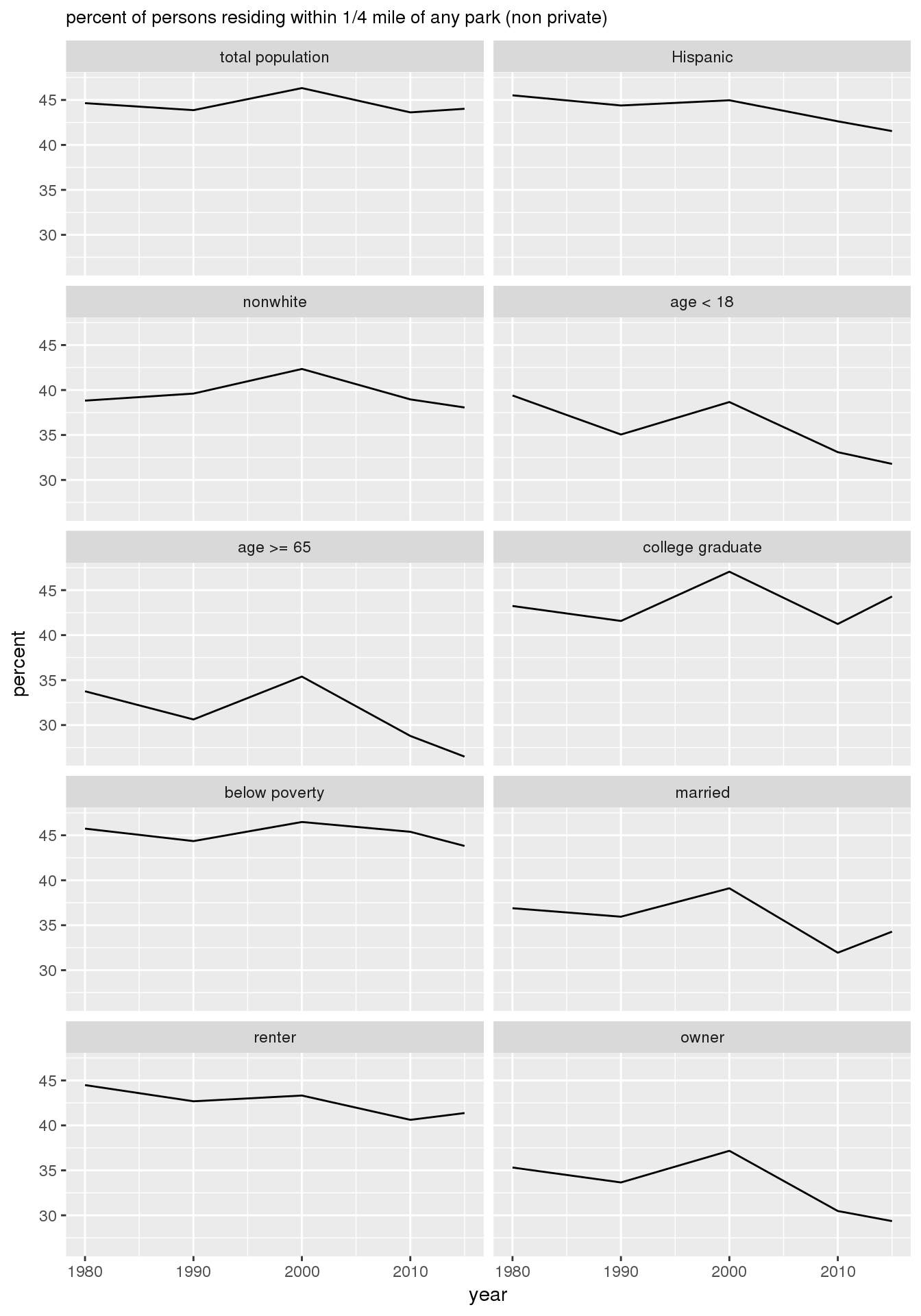
ggsave(filename = file.path(imagedir, "parks_noprivate_demographics.png"), plot = g, width = 4, height = 6, units = "in")All parks
sql <- "
with
--parks
prp as (select * from yakima_equity.park_private)
, p0 as (select * from yakima_equity.parksvalid where yearcreated <= xxxYEARxxx)
, p1 as (select the_geom_2286, st_area(the_geom_2286) as park_area_orig from p0)
--park buffer
, pb as (select true as buffer, st_union(st_buffer(the_geom_2286, 5280/4)) as p_geom from p1)
--annexation
, anx as (select st_union(the_geom_2286) as geom from yakima_equity.annexations where extract('year' from annex_date) <= xxxYEARxxx)
--non-buffer
, pnb as (select false as buffer, st_difference(anx.geom, pb.p_geom) as p_geom from pb, anx where st_intersects(anx.geom, pb.p_geom))
--combined
, p as (select * from pb union all select * from pnb)
--census tracts
, ct as (select st_area(the_geom_2286) as area_orig, * from yakima_equity.tract_xxxYEARxxx)
, cta as (select
tract
, total_pop
, age_lt_18
, age_lt_65
, age_ge_65
, median_hh_income
, median_family_income
, eth_hispanic
, race_nonwhite
, edu_collgrad
, edu_9th_somecoll
, edu_lt_9th
, pov_status
, pov_below_100pct
, married
, unmarried
, housingunits_renter
, housingunits_owner
from ct)
--clipped by anx
, ctanx as (select area_orig
, st_intersection(ct.the_geom_2286, anx.geom) as ctanx_geom
, tract
from ct, anx where st_intersects(ct.the_geom_2286, anx.geom))
--intersection of ctanx and parkbuf
, i as (select
st_area(st_intersection(ctanx.ctanx_geom, p.p_geom)) as area_clip
, *
from p, ctanx where st_intersects(p.p_geom, ctanx.ctanx_geom))
--ratio
, ir as (select tract, buffer, area_clip / area_orig as area_prop from i)
--proportional counts insid vs outside buffer
, props as (select tract, buffer
, total_pop * area_prop as total_pop
, age_lt_18 * area_prop as age_lt_18
, age_lt_65 * area_prop as age_lt_65
, age_ge_65 * area_prop as age_ge_65
, median_hh_income
, median_family_income
, eth_hispanic * area_prop as eth_hispanic
, race_nonwhite * area_prop as race_nonwhite
, edu_collgrad * area_prop as edu_collgrad
, edu_9th_somecoll * area_prop as edu_9th_somecoll
, edu_lt_9th * area_prop as edu_lt_9th
, pov_status * area_prop as pov_status
, pov_below_100pct * area_prop as pov_below_100pct
, married * area_prop as married
, unmarried * area_prop as unmarried
, housingunits_renter * area_prop as housingunits_renter
, housingunits_owner * area_prop as housingunits_owner
from ir left join cta using(tract))
--sum insie vs outside buffer
, ssum as (select
buffer
, sum(total_pop) as total_pop
, sum(eth_hispanic) as eth_hispanic
, sum(race_nonwhite) as race_nonwhite
, sum(age_lt_18) as age_lt_18
, sum(age_lt_65) as age_lt_65
, sum(age_ge_65) as age_ge_65
, sum(edu_collgrad) as edu_collgrad
, sum(edu_9th_somecoll) as edu_9th_somecoll
, sum(edu_lt_9th) as edu_lt_9th
, sum(pov_status) as pov_status
, sum(pov_below_100pct) as pov_below_100pct
, sum(married) as married
, sum(unmarried) as unmarried
, sum(housingunits_renter) as housingunits_renter
, sum(housingunits_owner ) as housingunits_owner
from props
group by buffer)
--proportion with access
, paxs as (select xxxYEARxxx::integer as year
, buffer
, 100 * total_pop / sum(total_pop) over() as total_pop
, 100 * eth_hispanic / sum(eth_hispanic) over() as eth_hispanic
, 100 * race_nonwhite / sum(race_nonwhite) over() as race_nonwhite
, 100 * age_lt_18 / sum(age_lt_18) over() as age_lt_18
, 100 * age_lt_65 / sum(age_lt_65) over() as age_lt_65
, 100 * age_ge_65 / sum(age_ge_65) over() as age_ge_65
, 100 * edu_collgrad / sum(edu_collgrad) over() as edu_collgrad
, 100 * edu_9th_somecoll / sum(edu_9th_somecoll) over() as edu_9th_somecoll
, 100 * edu_lt_9th / sum(edu_lt_9th) over() as edu_lt_9th
, 100 * pov_status / sum(pov_status) over() as pov_status
, 100 * pov_below_100pct / sum(pov_below_100pct) over() as pov_below_100pct
, 100 * married / sum(married) over() as married
, 100 * unmarried / sum(unmarried) over() as unmarried
, 100 * housingunits_renter / sum(housingunits_renter) over() as housingunits_renter
, 100 * housingunits_owner / sum(housingunits_owner ) over() as housingunits_owner
from ssum)
select * from paxs"
ydat <- NULL
for(y in c(1980, 1990, 2000, 2010, 2015)){
sqly <- gsub("xxxYEARxxx", y, sql)
ydat <- rbind(ydat, dbGetQuery(conn = dbconn, statement = sqly))
}
# drop some columns, rename some.
ydat$pov_status <- ydat$unmarried <- ydat$total_pop <- ydat$age_lt_65 <- ydat$edu_9th_somecoll <- ydat$edu_9th_somecoll <- NULL
names(ydat) <- c("year", "buffer", "total population", "Hispanic", "nonwhite", "age < 18", "age >= 65", "college graduate", "below poverty", "married", "renter", "owner")
# melt
ydatl <- ydatl0 <- melt(ydat, id.vars=c("year","buffer"), value.name = "percent")
# ydatl0$year <- factor(ydatl0$year)
# g <- ggplot(data = ydatl0, aes(x = year, y = percent, fill = buffer)) +
# geom_bar(position = "dodge", stat = "identity") +
# facet_wrap(~variable, ncol = 2) +
# scale_fill_discrete(name="in 1/4 mile buffer")
# print(g)
# ggsave(filename = file.path(imagedir, "parks_demographics_16th.png"), plot = g, width = ggsavewidth, height = ggsaveheight, units = "in")
ydatl <- ydatl[ydatl$buffer,]
g <- ggplot(data = ydatl, aes(x = year, y = percent)) +
geom_line() +
facet_wrap(~variable, ncol = 2) +
labs(title = "percent of persons residing within 1/4 mile of any park (all)") +
theme(plot.title = element_text(size=10))
print(g)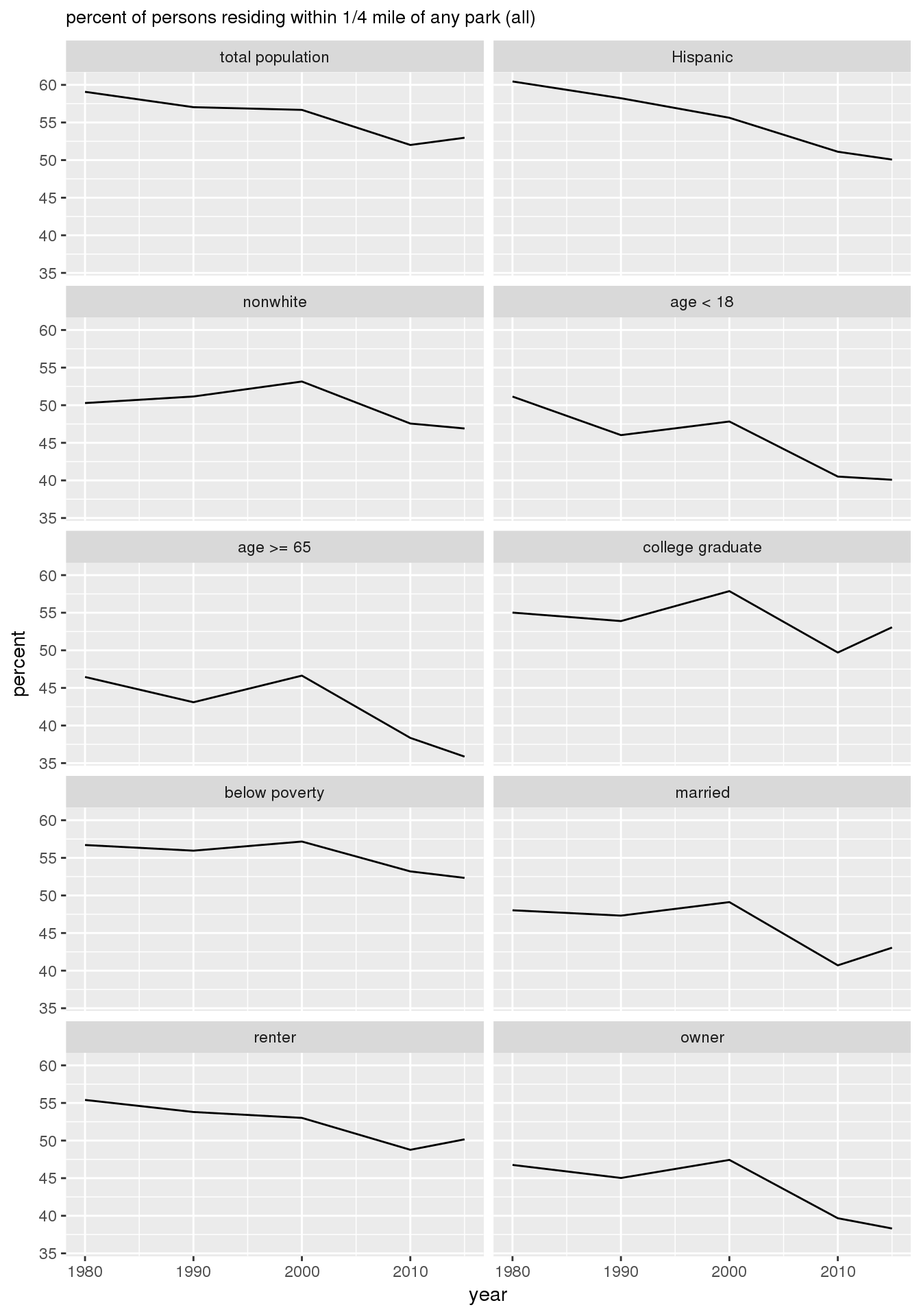
ggsave(filename = file.path(imagedir, "parks_all_demographics.png"), plot = g, width = 4, height = 6, units = "in")Furthermore, when stratified by 16th Avenue, there were more persons residing within 1/4 mile of park on the east side than on the west side.
Parks with no private funding
sql <- "
with
--parks
prp as (select * from yakima_equity.park_private)
, p0 as (select * from yakima_equity.parksvalid where yearcreated <= xxxYEARxxx and name not in (select name from prp))
, p1 as (select the_geom_2286, st_area(the_geom_2286) as park_area_orig from p0)
--annexation
, anx as (select st_union(the_geom_2286) as geom from yakima_equity.annexations where extract('year' from annex_date) <= xxxYEARxxx)
--park buffer
, pb0 as (select true as buffer, st_union(st_buffer(the_geom_2286, 5280/4)) as geom from p1)
----clip by annexation
, pb as (select buffer, (st_multi(st_intersection(pb0.geom, anx.geom)))::geometry(multipolygon, 2286) as geom from pb0, anx where st_intersects(pb0.geom, anx.geom))
--e/w
, ew as (select zone_16th, the_geom_2286 as geom from yakima_equity.ew_16th)
--non-buffer
, pnb as (select false as buffer, (st_multi(st_difference(anx.geom, pb.geom)))::geometry(multipolygon, 2286) as geom from pb, anx where st_intersects(anx.geom, pb.geom))
--combined
, pb_pnb as (select * from pb union all select * from pnb)
--overlay e/w --note use of polygonalintersection function
, pball as (select buffer, zone_16th, polygonalintersection(ew.geom, pb_pnb.geom, 2286) as geom from ew, pb_pnb)
--census tracts
, ct as (select the_geom_2286 as geom, tract::text from yakima_equity.tract_xxxYEARxxx)
--attributes only
, cta as (select
tract::text
, st_area(the_geom_2286) as area_orig
, total_pop
, age_lt_18
, age_lt_65
, age_ge_65
, median_hh_income
, median_family_income
, eth_hispanic
, race_nonwhite
, edu_collgrad
, edu_9th_somecoll
, edu_lt_9th
, pov_status
, pov_below_100pct
, married
, unmarried
, housingunits_renter
, housingunits_owner
from yakima_equity.tract_xxxYEARxxx)
--intersection of ct and pball
, i0 as (select
polygonalintersection(ct.geom, pball.geom, 2286) as geom
, st_area(st_intersection(ct.geom, pball.geom)) as area_int
, buffer
, zone_16th
, tract
from pball, ct where st_intersects(pball.geom, ct.geom))
, i as (select
area_int
, buffer
, zone_16th
, tract::text
--ratio
, area_int / area_orig as area_prop
from i0 join cta using (tract) where area_int > 0)
--proportional counts inside vs outside buffer
, props as (select tract, buffer, zone_16th
, total_pop * area_prop as total_pop
, age_lt_18 * area_prop as age_lt_18
, age_lt_65 * area_prop as age_lt_65
, age_ge_65 * area_prop as age_ge_65
, median_hh_income
, median_family_income
, eth_hispanic * area_prop as eth_hispanic
, race_nonwhite * area_prop as race_nonwhite
, edu_collgrad * area_prop as edu_collgrad
, edu_9th_somecoll * area_prop as edu_9th_somecoll
, edu_lt_9th * area_prop as edu_lt_9th
, pov_status * area_prop as pov_status
, pov_below_100pct * area_prop as pov_below_100pct
, married * area_prop as married
, unmarried * area_prop as unmarried
, housingunits_renter * area_prop as housingunits_renter
, housingunits_owner * area_prop as housingunits_owner
from i join cta using(tract))
-- select * from props order by tract, buffer
--sum insie vs outside buffer
, ssum as (select
buffer
, zone_16th
, sum(total_pop) as total_pop
, sum(eth_hispanic) as eth_hispanic
, sum(race_nonwhite) as race_nonwhite
, sum(age_lt_18) as age_lt_18
, sum(age_lt_65) as age_lt_65
, sum(age_ge_65) as age_ge_65
, sum(edu_collgrad) as edu_collgrad
, sum(edu_9th_somecoll) as edu_9th_somecoll
, sum(edu_lt_9th) as edu_lt_9th
, sum(pov_status) as pov_status
, sum(pov_below_100pct) as pov_below_100pct
, sum(married) as married
, sum(unmarried) as unmarried
, sum(housingunits_renter) as housingunits_renter
, sum(housingunits_owner ) as housingunits_owner
from props
group by buffer, zone_16th)
--proportion with access
, paxs as (select xxxYEARxxx::integer as year
, buffer
, zone_16th
, 100 * total_pop / sum(total_pop) over() as total_pop
, 100 * eth_hispanic / sum(eth_hispanic) over() as eth_hispanic
, 100 * race_nonwhite / sum(race_nonwhite) over() as race_nonwhite
, 100 * age_lt_18 / sum(age_lt_18) over() as age_lt_18
, 100 * age_lt_65 / sum(age_lt_65) over() as age_lt_65
, 100 * age_ge_65 / sum(age_ge_65) over() as age_ge_65
, 100 * edu_collgrad / sum(edu_collgrad) over() as edu_collgrad
, 100 * edu_9th_somecoll / sum(edu_9th_somecoll) over() as edu_9th_somecoll
, 100 * edu_lt_9th / sum(edu_lt_9th) over() as edu_lt_9th
, 100 * pov_status / sum(pov_status) over() as pov_status
, 100 * pov_below_100pct / sum(pov_below_100pct) over() as pov_below_100pct
, 100 * married / sum(married) over() as married
, 100 * unmarried / sum(unmarried) over() as unmarried
, 100 * housingunits_renter / sum(housingunits_renter) over() as housingunits_renter
, 100 * housingunits_owner / sum(housingunits_owner ) over() as housingunits_owner
from ssum)
select * from paxs;"
ydat <- NULL
for(y in c(1980, 1990, 2000, 2010, 2015)){
sqly <- gsub("xxxYEARxxx", y, sql)
ydat <- rbind(ydat, dbGetQuery(conn = dbconn, statement = sqly))
}
# drop some columns, rename some.
ydat$pov_status <- ydat$unmarried <- ydat$total_pop <- ydat$age_lt_65 <- ydat$edu_9th_somecoll <- ydat$edu_9th_somecoll <- NULL
names(ydat) <- c("year", "buffer", "zone_16th", "total population", "Hispanic", "nonwhite", "age < 18", "age >= 65", "college graduate", "below poverty", "married", "renter", "owner")
# melt
ydatl <- ydatl0 <- melt(ydat, id.vars=c("year","buffer","zone_16th"), value.name = "percent")
# ydatl0$year <- factor(ydatl0$year)
# g <- ggplot(data = ydatl0, aes(x = year, y = percent, fill = buffer)) +
# geom_bar(position = "dodge", stat = "identity") +
# facet_wrap(~variable, ncol = 2) +
# scale_fill_discrete(name="in 1/4 mile buffer")
# print(g)
# ggsave(filename = file.path(imagedir, "parks_demographics_16th.png"), plot = g, width = ggsavewidth, height = ggsaveheight, units = "in")
ydatl <- ydatl[ydatl$buffer,]
l <- levels(ydatl$variable)
lx <- gsub(" ", "\n", l)
ydatl$vname <- factor(gsub(" ", "\n", ydatl$variable), levels = lx)
#ydatl$year <- factor(ydatl$year)
g <- ggplot(data = ydatl, aes(x = year, y = percent)) +
geom_line() +
#facet_wrap(variable ~ zone_16th, ncol = 2) +
facet_grid(vname ~ zone_16th) +
labs(title = "percent of persons residing within 1/4 mile of any park (non private)") +
theme(plot.title = element_text(size=10))
print(g)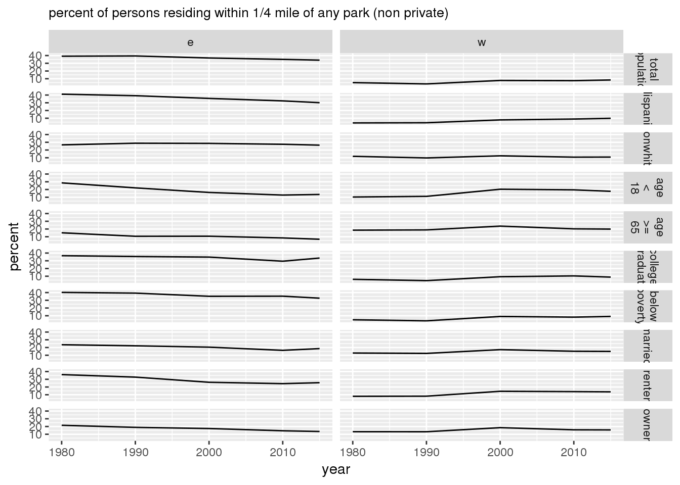
ggsave(filename = file.path(imagedir, "parks_noprivate_demographics_16th.png"), plot = g, width = 4, height = 8, units = "in")All parks
sql <- "
with
--parks
prp as (select * from yakima_equity.park_private)
, p0 as (select * from yakima_equity.parksvalid where yearcreated <= xxxYEARxxx)
, p1 as (select the_geom_2286, st_area(the_geom_2286) as park_area_orig from p0)
--annexation
, anx as (select st_union(the_geom_2286) as geom from yakima_equity.annexations where extract('year' from annex_date) <= xxxYEARxxx)
--park buffer
, pb0 as (select true as buffer, st_union(st_buffer(the_geom_2286, 5280/4)) as geom from p1)
----clip by annexation
, pb as (select buffer, (st_multi(st_intersection(pb0.geom, anx.geom)))::geometry(multipolygon, 2286) as geom from pb0, anx where st_intersects(pb0.geom, anx.geom))
--e/w
, ew as (select zone_16th, the_geom_2286 as geom from yakima_equity.ew_16th)
--non-buffer
, pnb as (select false as buffer, (st_multi(st_difference(anx.geom, pb.geom)))::geometry(multipolygon, 2286) as geom from pb, anx where st_intersects(anx.geom, pb.geom))
--combined
, pb_pnb as (select * from pb union all select * from pnb)
--overlay e/w --note use of polygonalintersection function
, pball as (select buffer, zone_16th, polygonalintersection(ew.geom, pb_pnb.geom, 2286) as geom from ew, pb_pnb)
--census tracts
, ct as (select the_geom_2286 as geom, tract::text from yakima_equity.tract_xxxYEARxxx)
--attributes only
, cta as (select
tract::text
, st_area(the_geom_2286) as area_orig
, total_pop
, age_lt_18
, age_lt_65
, age_ge_65
, median_hh_income
, median_family_income
, eth_hispanic
, race_nonwhite
, edu_collgrad
, edu_9th_somecoll
, edu_lt_9th
, pov_status
, pov_below_100pct
, married
, unmarried
, housingunits_renter
, housingunits_owner
from yakima_equity.tract_xxxYEARxxx)
--intersection of ct and pball
, i0 as (select
polygonalintersection(ct.geom, pball.geom, 2286) as geom
, st_area(st_intersection(ct.geom, pball.geom)) as area_int
, buffer
, zone_16th
, tract
from pball, ct where st_intersects(pball.geom, ct.geom))
, i as (select
area_int
, buffer
, zone_16th
, tract::text
--ratio
, area_int / area_orig as area_prop
from i0 join cta using (tract) where area_int > 0)
--proportional counts inside vs outside buffer
, props as (select tract, buffer, zone_16th
, total_pop * area_prop as total_pop
, age_lt_18 * area_prop as age_lt_18
, age_lt_65 * area_prop as age_lt_65
, age_ge_65 * area_prop as age_ge_65
, median_hh_income
, median_family_income
, eth_hispanic * area_prop as eth_hispanic
, race_nonwhite * area_prop as race_nonwhite
, edu_collgrad * area_prop as edu_collgrad
, edu_9th_somecoll * area_prop as edu_9th_somecoll
, edu_lt_9th * area_prop as edu_lt_9th
, pov_status * area_prop as pov_status
, pov_below_100pct * area_prop as pov_below_100pct
, married * area_prop as married
, unmarried * area_prop as unmarried
, housingunits_renter * area_prop as housingunits_renter
, housingunits_owner * area_prop as housingunits_owner
from i join cta using(tract))
-- select * from props order by tract, buffer
--sum insie vs outside buffer
, ssum as (select
buffer
, zone_16th
, sum(total_pop) as total_pop
, sum(eth_hispanic) as eth_hispanic
, sum(race_nonwhite) as race_nonwhite
, sum(age_lt_18) as age_lt_18
, sum(age_lt_65) as age_lt_65
, sum(age_ge_65) as age_ge_65
, sum(edu_collgrad) as edu_collgrad
, sum(edu_9th_somecoll) as edu_9th_somecoll
, sum(edu_lt_9th) as edu_lt_9th
, sum(pov_status) as pov_status
, sum(pov_below_100pct) as pov_below_100pct
, sum(married) as married
, sum(unmarried) as unmarried
, sum(housingunits_renter) as housingunits_renter
, sum(housingunits_owner ) as housingunits_owner
from props
group by buffer, zone_16th)
--proportion with access
, paxs as (select xxxYEARxxx::integer as year
, buffer
, zone_16th
, 100 * total_pop / sum(total_pop) over() as total_pop
, 100 * eth_hispanic / sum(eth_hispanic) over() as eth_hispanic
, 100 * race_nonwhite / sum(race_nonwhite) over() as race_nonwhite
, 100 * age_lt_18 / sum(age_lt_18) over() as age_lt_18
, 100 * age_lt_65 / sum(age_lt_65) over() as age_lt_65
, 100 * age_ge_65 / sum(age_ge_65) over() as age_ge_65
, 100 * edu_collgrad / sum(edu_collgrad) over() as edu_collgrad
, 100 * edu_9th_somecoll / sum(edu_9th_somecoll) over() as edu_9th_somecoll
, 100 * edu_lt_9th / sum(edu_lt_9th) over() as edu_lt_9th
, 100 * pov_status / sum(pov_status) over() as pov_status
, 100 * pov_below_100pct / sum(pov_below_100pct) over() as pov_below_100pct
, 100 * married / sum(married) over() as married
, 100 * unmarried / sum(unmarried) over() as unmarried
, 100 * housingunits_renter / sum(housingunits_renter) over() as housingunits_renter
, 100 * housingunits_owner / sum(housingunits_owner ) over() as housingunits_owner
from ssum)
select * from paxs;"
ydat <- NULL
for(y in c(1980, 1990, 2000, 2010, 2015)){
sqly <- gsub("xxxYEARxxx", y, sql)
ydat <- rbind(ydat, dbGetQuery(conn = dbconn, statement = sqly))
}
# drop some columns, rename some.
ydat$pov_status <- ydat$unmarried <- ydat$total_pop <- ydat$age_lt_65 <- ydat$edu_9th_somecoll <- ydat$edu_9th_somecoll <- NULL
names(ydat) <- c("year", "buffer", "zone_16th", "total population", "Hispanic", "nonwhite", "age < 18", "age >= 65", "college graduate", "below poverty", "married", "renter", "owner")
# melt
ydatl <- ydatl0 <- melt(ydat, id.vars=c("year","buffer","zone_16th"), value.name = "percent")
# ydatl0$year <- factor(ydatl0$year)
# g <- ggplot(data = ydatl0, aes(x = year, y = percent, fill = buffer)) +
# geom_bar(position = "dodge", stat = "identity") +
# facet_wrap(~variable, ncol = 2) +
# scale_fill_discrete(name="in 1/4 mile buffer")
# print(g)
# ggsave(filename = file.path(imagedir, "parks_demographics_16th.png"), plot = g, width = ggsavewidth, height = ggsaveheight, units = "in")
ydatl <- ydatl[ydatl$buffer,]
l <- levels(ydatl$variable)
lx <- gsub(" ", "\n", l)
ydatl$vname <- factor(gsub(" ", "\n", ydatl$variable), levels = lx)
#ydatl$year <- factor(ydatl$year)
g <- ggplot(data = ydatl, aes(x = year, y = percent)) +
geom_line() +
#facet_wrap(variable ~ zone_16th, ncol = 2) +
facet_grid(vname ~ zone_16th) +
labs(title = "percent of persons residing within 1/4 mile of any park (all)") +
theme(plot.title = element_text(size=10))
print(g)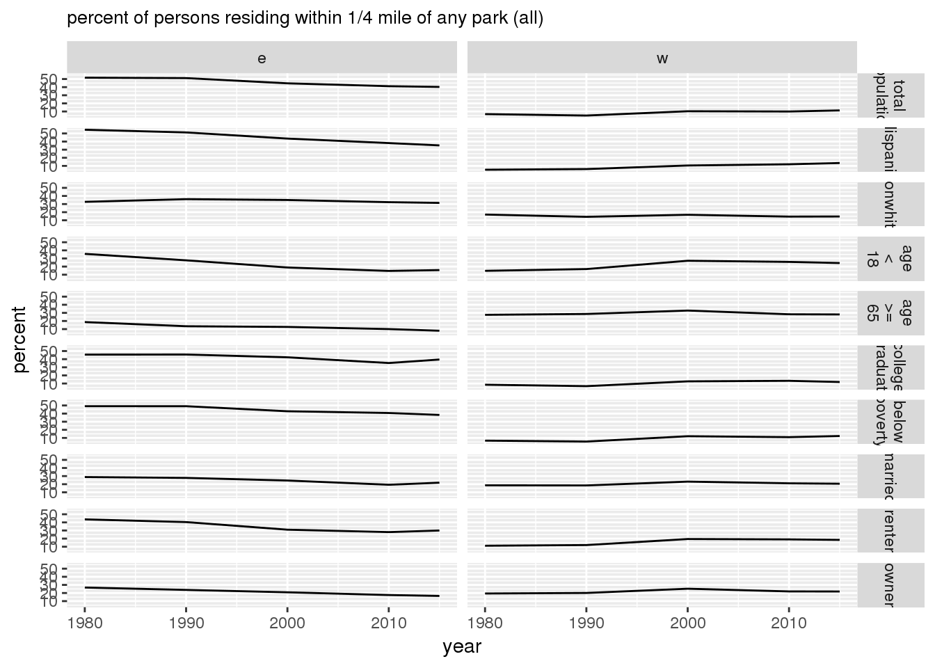
ggsave(filename = file.path(imagedir, "parks_all_demographics_16th.png"), plot = g, width = 4, height = 8, units = "in")3.4 Built environment
for(i in (ncol(citysum) - 1):ncol(citysum)){
                                colname <- colnames(citysum)[i]
                                title <- titles[i]
                                ylab <- switch(substr(colname, 1, 3),
                                    med="$",
                                    pct="percent",
                                    pro="$",
                                    yea="year")

                                g <- ggplot(data = citysum, aes(factor(year), citysum[,i])) + geom_bar(stat = "identity") + labs(x="year", y=ylab, title=title) +
                                theme(plot.title = element_text(size=12))

                                if(colname=='year_built'){
                                    g <- g + coord_cartesian(ylim = c(1940, 1970))
                                }
                                if(colname=='propvalue'){
                                    g <- g + coord_cartesian(ylim = c(150000, 250000))
                                }
                                print(g)
                                ggsave(filename = file.path(imagedir, sprintf("%s.png", colname)), plot = g, width = ggsavewidth, height = ggsaveheight, units = "in")
                            }
for(i in (ncol(ewsum)-1):ncol(ewsum)){
                                colname <- colnames(ewsum)[i]
                                title <- titles[i]
                                ylab <- switch(substr(colname, 1, 3),
                                med="$",
                                pct="percent",
                                pro="$",
                                yea="year")

                                g <- ggplot(data = ewsum, aes(factor(year), ewsum[,i], fill=zone_16th)) + geom_bar(stat = "identity", position = "dodge") + labs(x="year", y=ylab, title=title, fill="16th Ave divide") +
                                theme(plot.title = element_text(size=12))

                                if(colname=='year_built'){
                                    g <- g + coord_cartesian(ylim = c(1940, 1970))
                                }
                                if(colname=='propvalue'){
                                    g <- g + coord_cartesian(ylim = c(150000, 250000))
                                }
                                print(g)
                                ggsave(filename = file.path(imagedir, sprintf("%s_16th.png", colname)), plot = g, width = ggsavewidth, height = ggsaveheight, units = "in")

                            }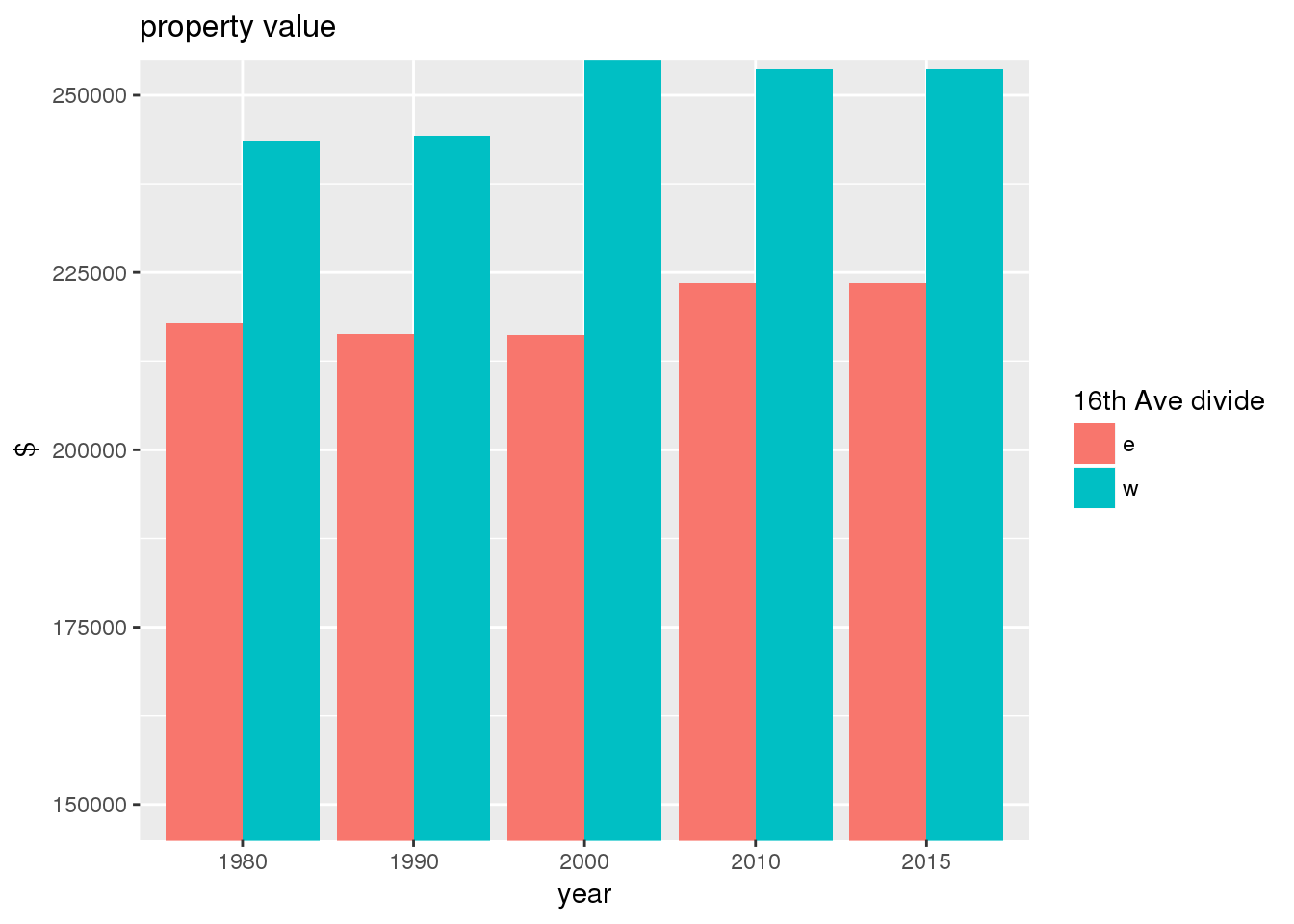
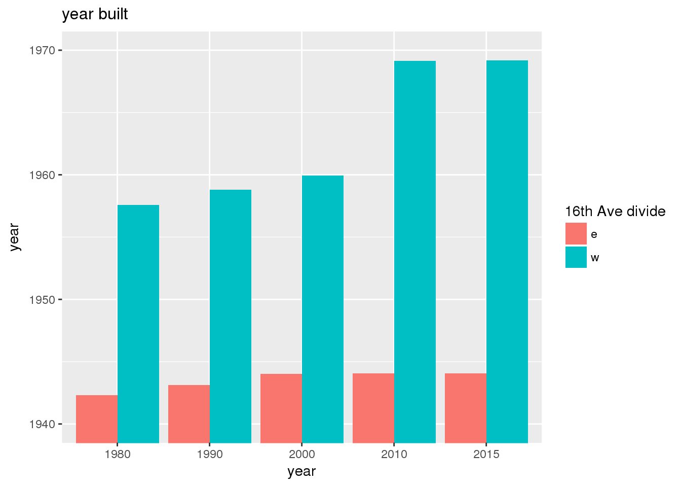
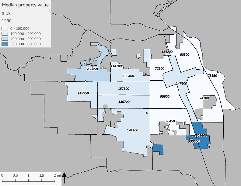
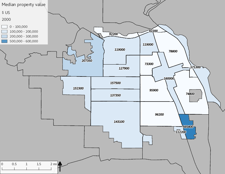
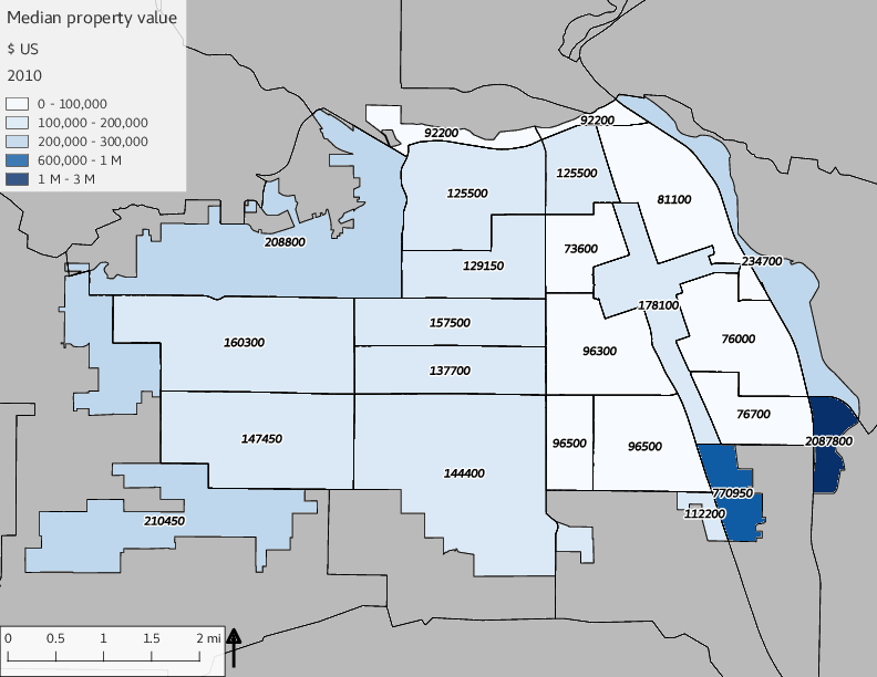
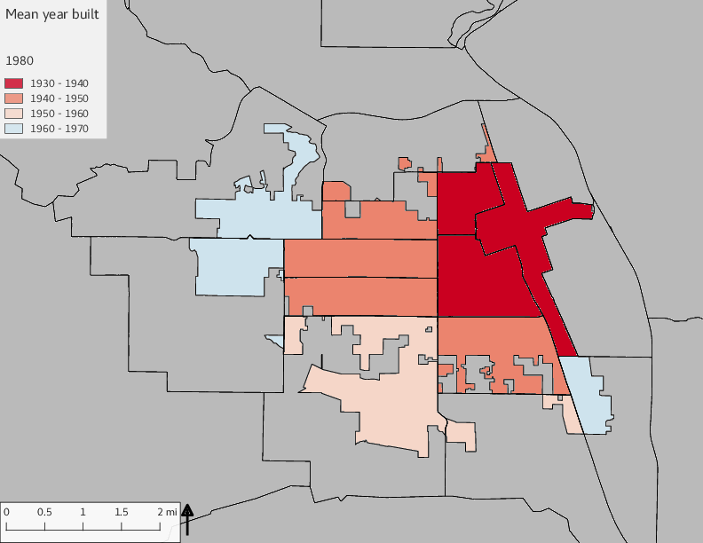
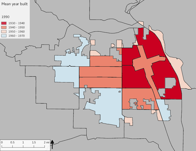
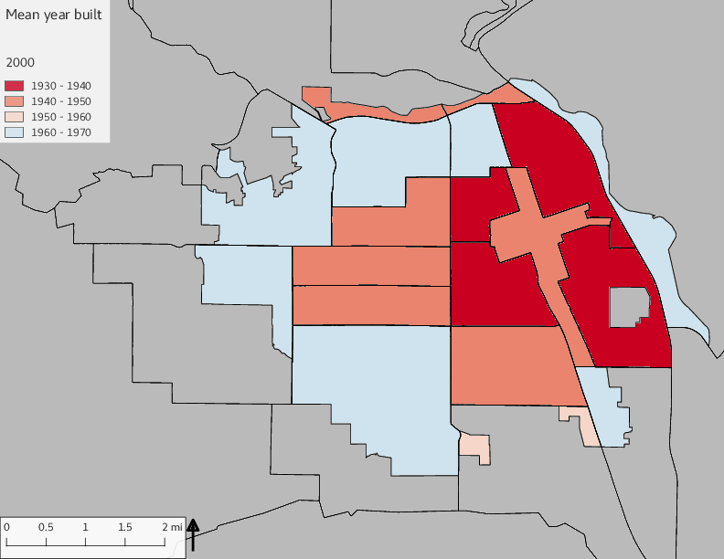
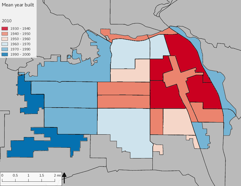
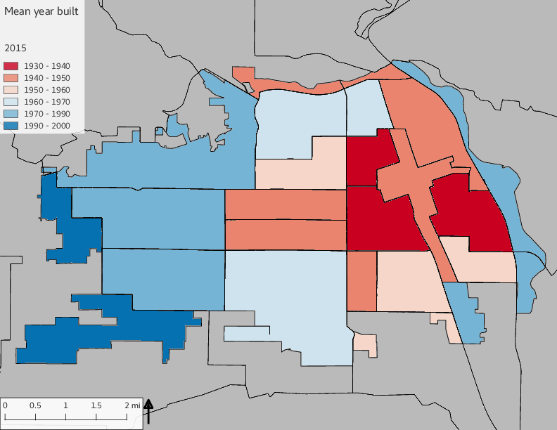
The set of built environment maps show changes in median property value and mean year built over time. The property value maps have the median value printed on each tract.
include_graphics(bemaps)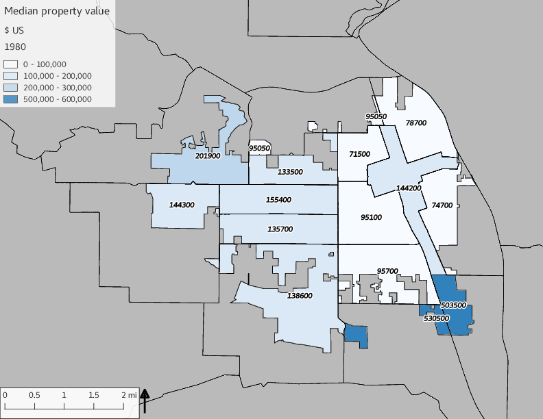

3.5 Current infrastructure allocation
The data in this section represent the most recent GIS data from YC and US Census data from 2015.
3.5.1 Public safety calls for service
It should be noted that no information was provided on response times ,so no analysis was possible. Also, given that there were 140 call types, no analysis was performed on any specific call type.
3.5.1.1 Police Department
sql <- "
with
--substitute input table and where clause
p as (select the_geom_2286, callsforservice_opened as opened, callsforservice_closed as closed, extract(epoch from callsforservice_closed - callsforservice_opened)/60 as response_cycle_minutes from yakima_equity.ykpdcfs)
--census tracts
, ct as (select st_area(the_geom_2286) as area_ct, * from yakima_equity.tract_2015)
--population east vs west
, tpop as (select zone_16th, sum(total_pop) as total_pop from ct group by zone_16th)
--intersect points and tracts
, px as (select opened, closed, response_cycle_minutes, zone_16th from ct, p where st_intersects(p.the_geom_2286, ct.the_geom_2286))
, px2 as (select * from px join tpop using(zone_16th))
--select * from f;
select * from px2"
pdcalls_resp <- dbGetQuery(conn = dbconn, statement = sql)
minpddate <- as.Date(min(pdcalls_resp$opened))
maxpddate <- as.Date(max(pdcalls_resp$closed))
ew_sum_pdcalls <- sqldf("with a as (select zone_16th, total_pop, round(avg(response_cycle_minutes)::numeric, 1) as avg_response_cycle_minutes, round(stddev(response_cycle_minutes)::numeric, 1) as sd_response_cycle_minutes, count(*) from pdcalls_resp group by zone_16th, total_pop order by zone_16th) select *, count / total_pop as calls_per_capita from a;")
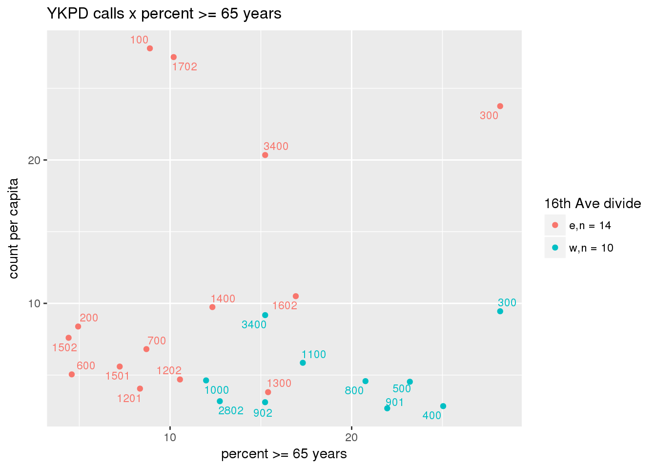
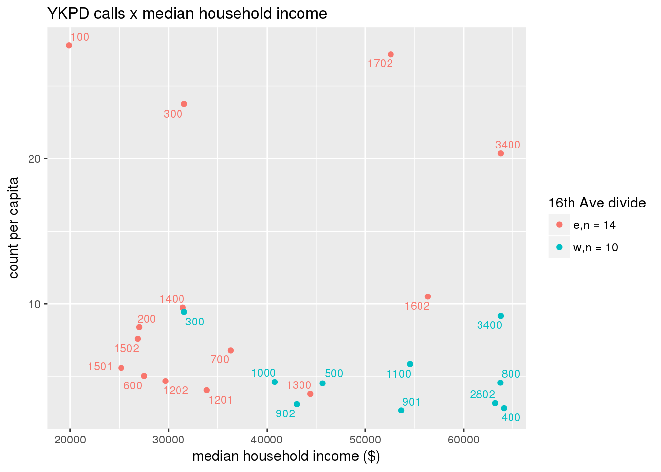
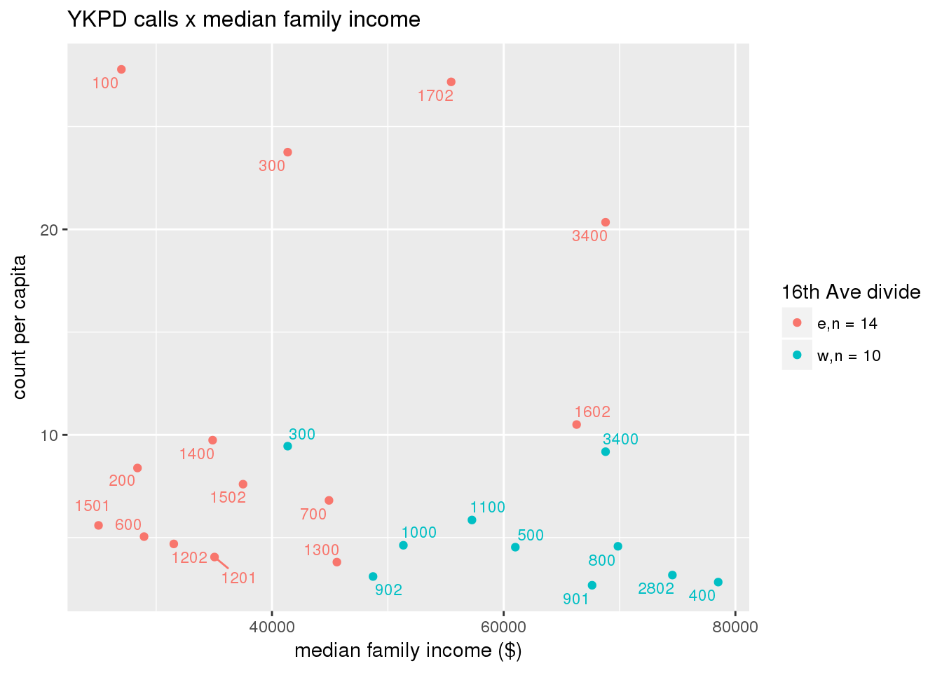
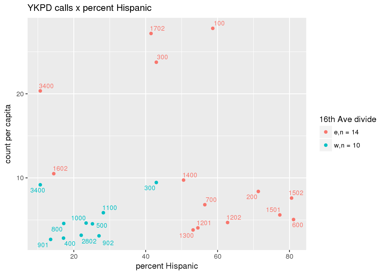
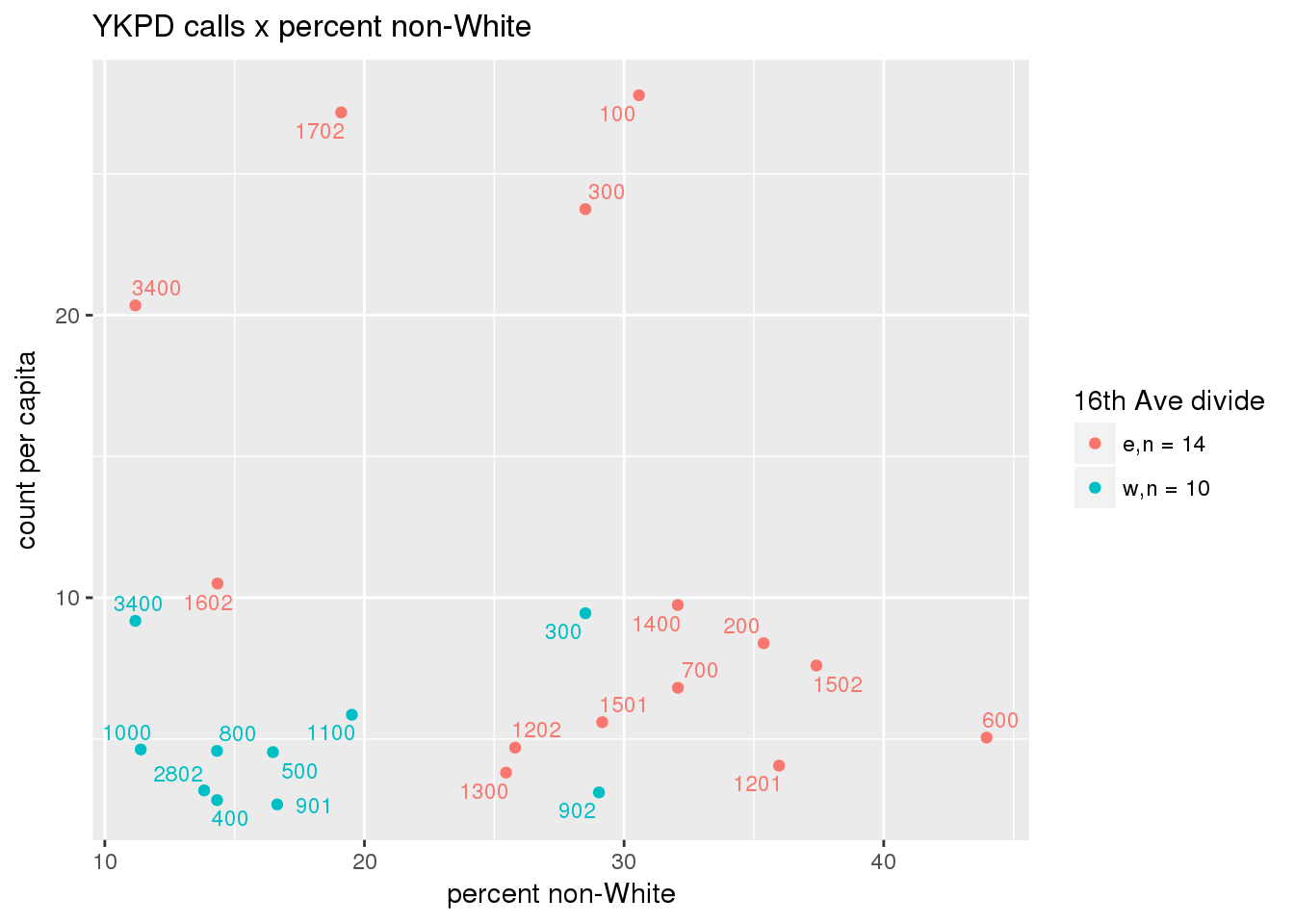
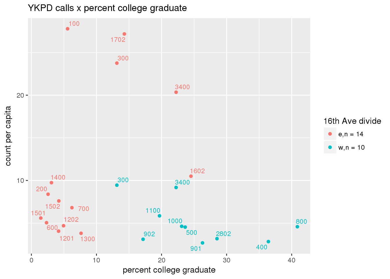
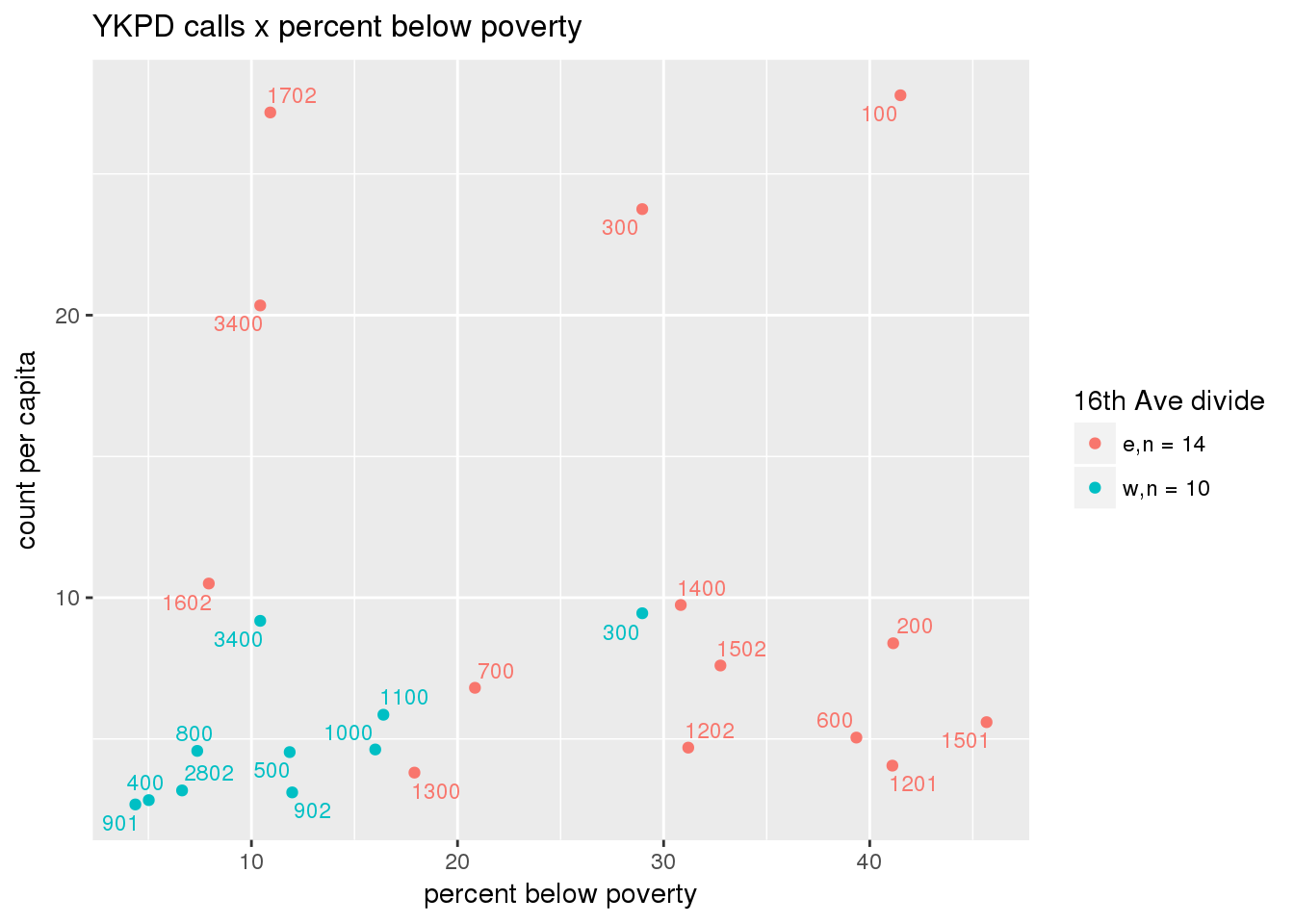
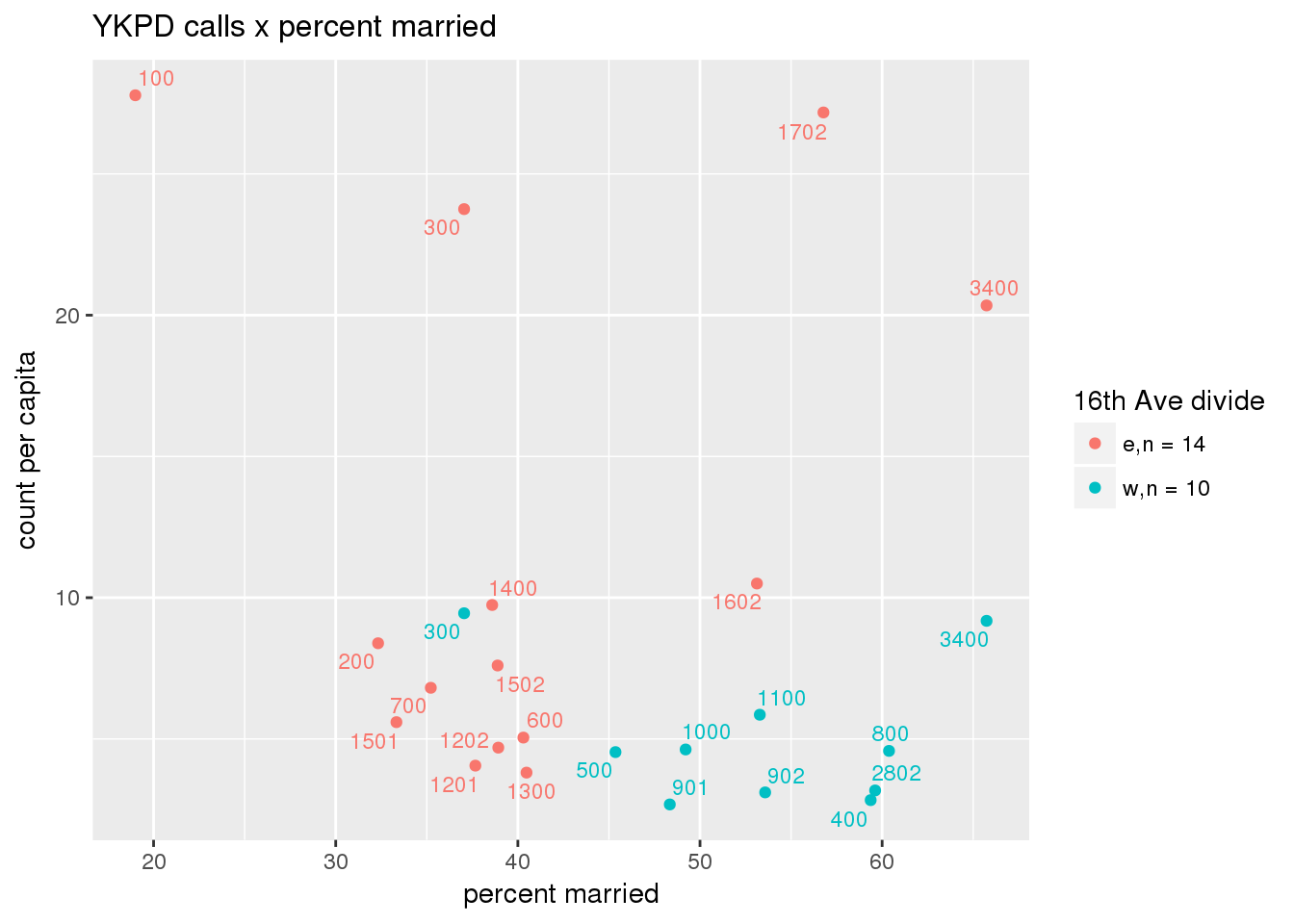
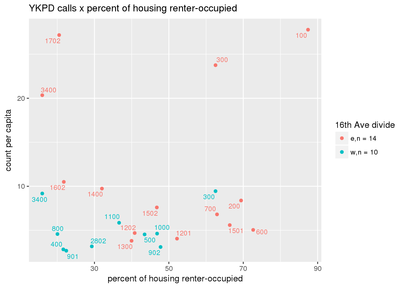
pdew <- split(ew_sum_pdcalls, ew_sum_pdcalls$zone_16th)Count of Police Department calls (n = 534566 from 2010-12-08 to 2017-09-11 were stratified by 16th Avenue as well as overlain on Census tracts. There were 364,166 calls (7.6 per capita) from the area east of 16th Avenue, and 170,400 calls (4.1 per capita) from the west side. There were no apparent patterns with respect to counts of calls per capita and Census demographic characteristics, either as a whole or with stratification by 16th Avenue. There are several census tracts on the east side with quite higher per capita calls, a situation that potentially warrants further investigation.
# count per capita pdcalls <- ptfcn(pttablename = "ykpdcfs", normvar = "capita", mytitle = "YKPD calls", legend_title = "16th Ave divide")
3.5.1.2 Fire Department
sql <- "
with
--substitute input table and where clause
p as (select the_geom_2286, callsforservice_opened as opened, callsforservice_closed as closed, extract(epoch from callsforservice_closed - callsforservice_opened)/60 as response_cycle_minutes from yakima_equity.ykfdcfs)
--census tracts
, ct as (select st_area(the_geom_2286) as area_ct, * from yakima_equity.tract_2015)
--population east vs west
, tpop as (select zone_16th, sum(total_pop) as total_pop from ct group by zone_16th)
--intersect points and tracts
, px as (select opened, closed, response_cycle_minutes, zone_16th from ct, p where st_intersects(p.the_geom_2286, ct.the_geom_2286))
, px2 as (select * from px join tpop using(zone_16th))
--select * from f;
select * from px2"
fdcalls_resp <- dbGetQuery(conn = dbconn, statement = sql)
minfddate <- as.Date(min(fdcalls_resp$opened))
maxfddate <- as.Date(max(fdcalls_resp$closed))
ew_sum_fdcalls <- sqldf("with a as (select zone_16th, total_pop, round(avg(response_cycle_minutes)::numeric, 1) as avg_response_cycle_minutes, round(stddev(response_cycle_minutes)::numeric, 1) as sd_response_cycle_minutes, count(*) from fdcalls_resp group by zone_16th, total_pop order by zone_16th) select *, count / total_pop as calls_per_capita from a;")
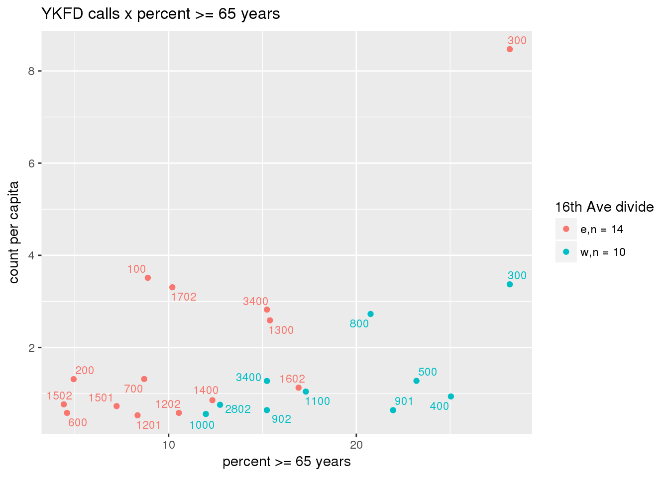
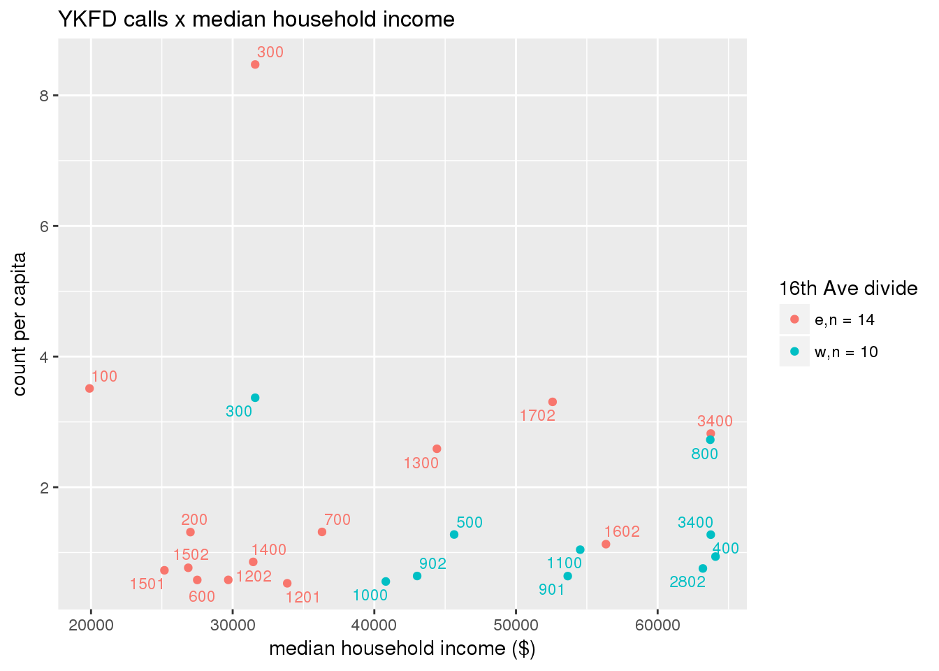
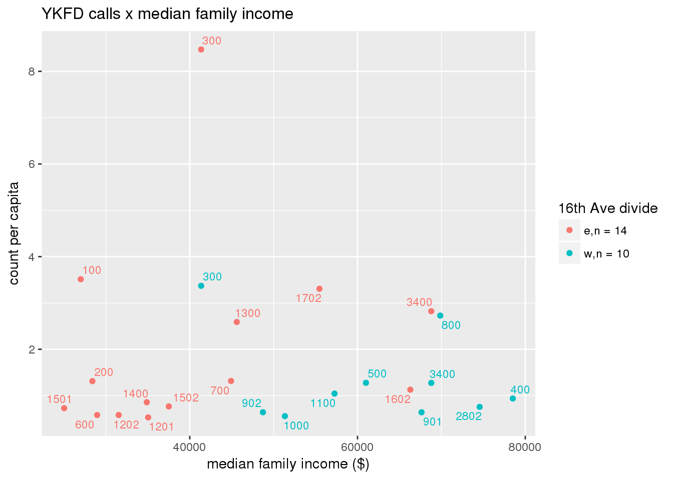
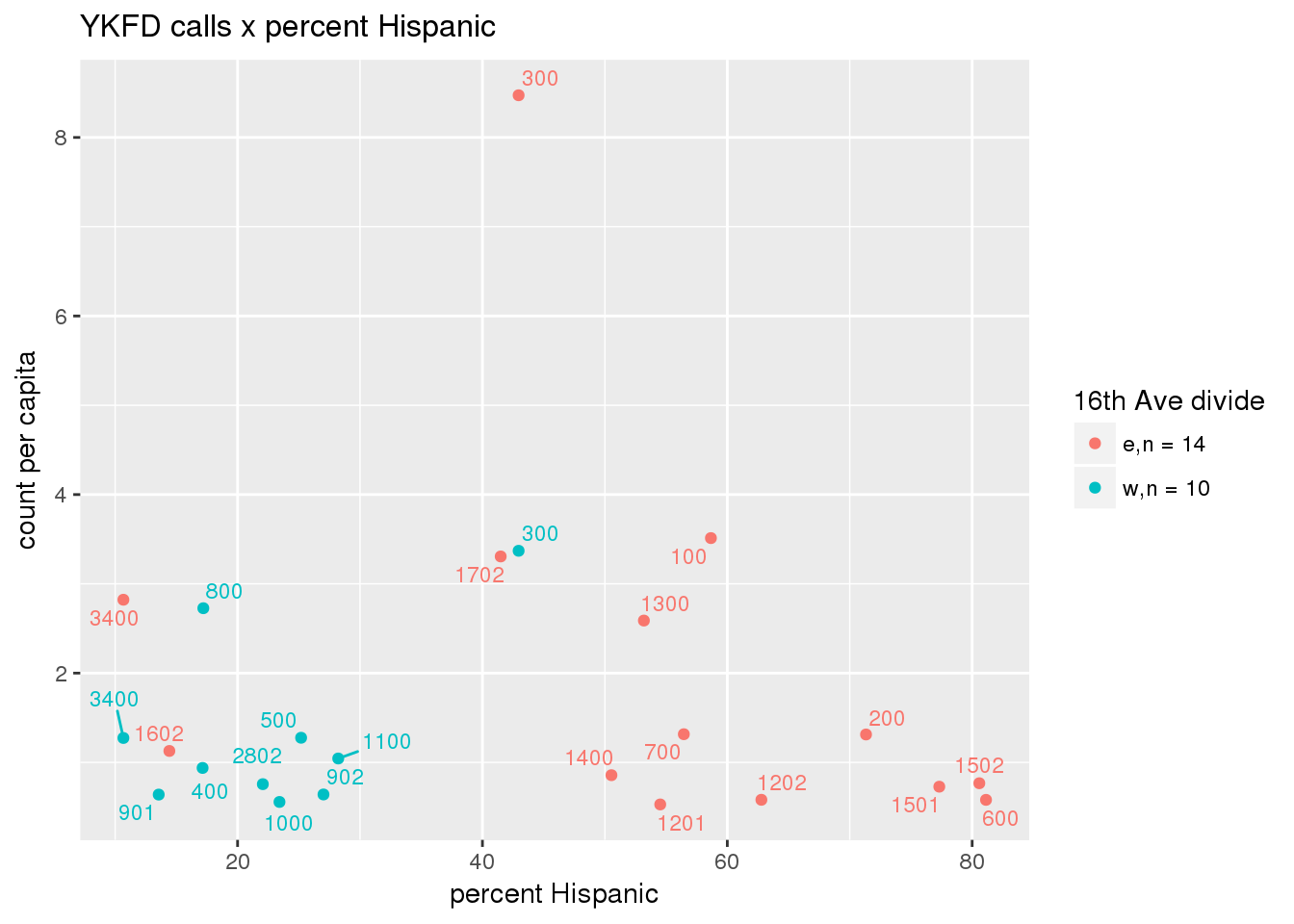
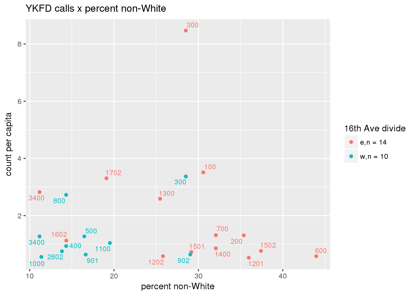
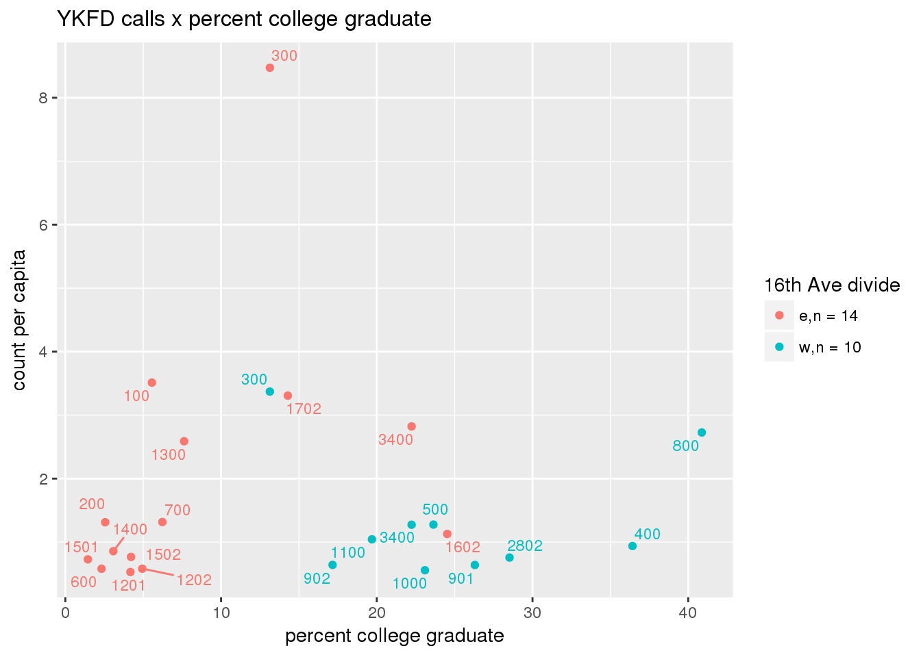
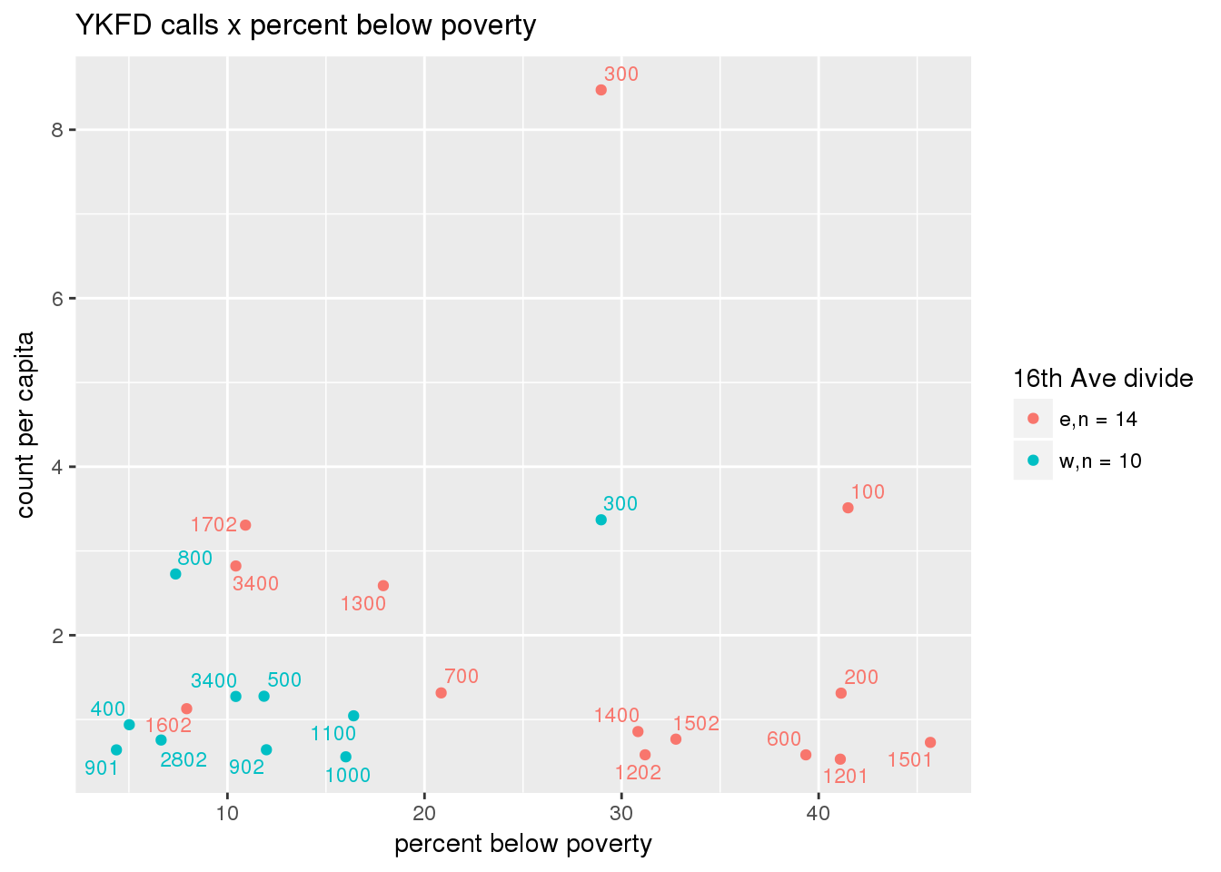
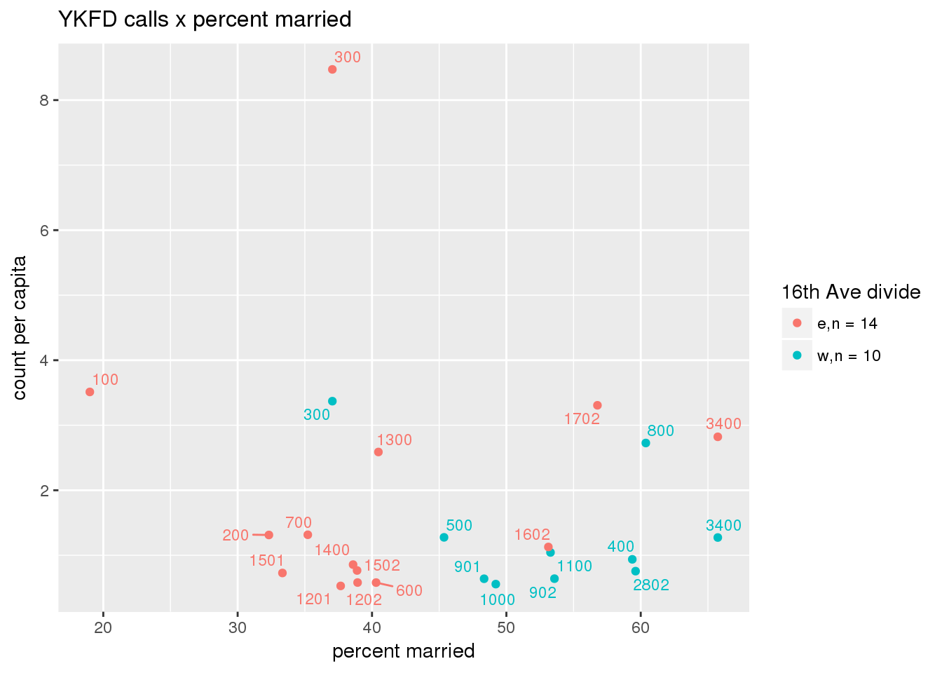
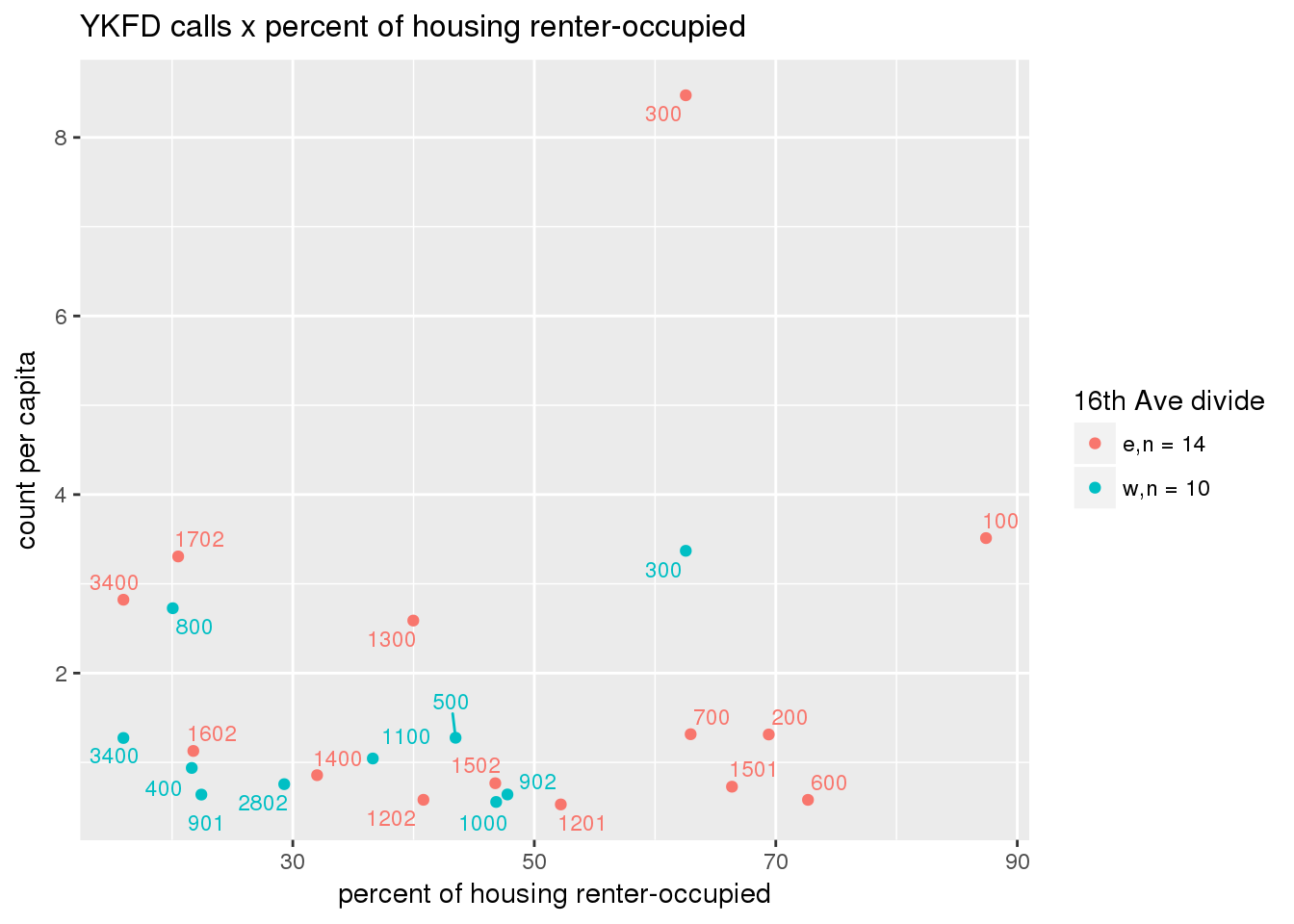
fdew <- split(ew_sum_fdcalls, ew_sum_fdcalls$zone_16th)Fire Department calls were nearly evenly split, with 50,223 calls (1 per capita) from the area east of 16th Avenue, and 49,332 calls (1.2 per capita) from the west side. Response cycle times were nearly 10 minutes shorter on the east side, with a mean of 37.8 minutes (SD=42.5) versus 48.4 minutes (SD = 58.8) on the west side. There were no apparent patterns with respect to counts of calls per capita and Census demographic characteristics, either as a whole or with stratification by 16th Avenue. However, there is a single tract with > 8 calls per capita, which is twice as high as the next highest tracts; this is a situation that probably warrants further investigation.
fdcalls <- ptfcn(pttablename = "ykfdcfs", normvar = "capita", mytitle = "YKFD calls", legend_title = "16th Ave divide")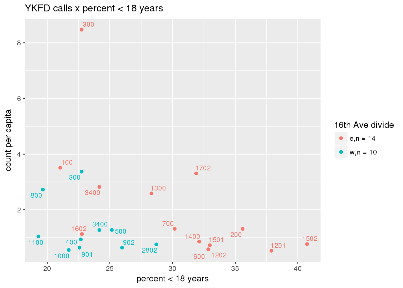
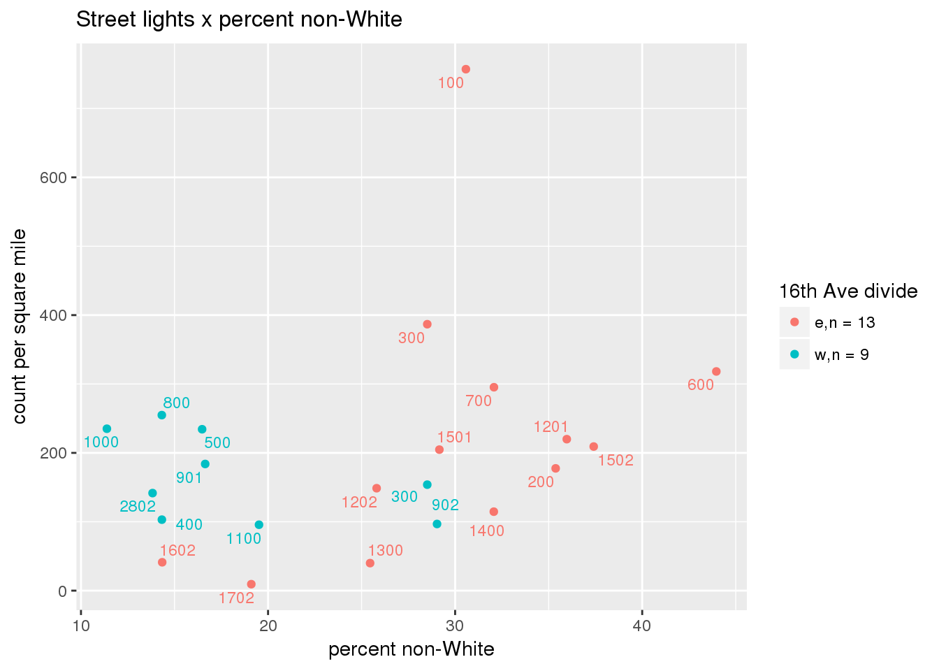
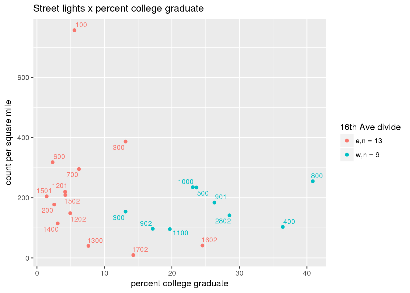
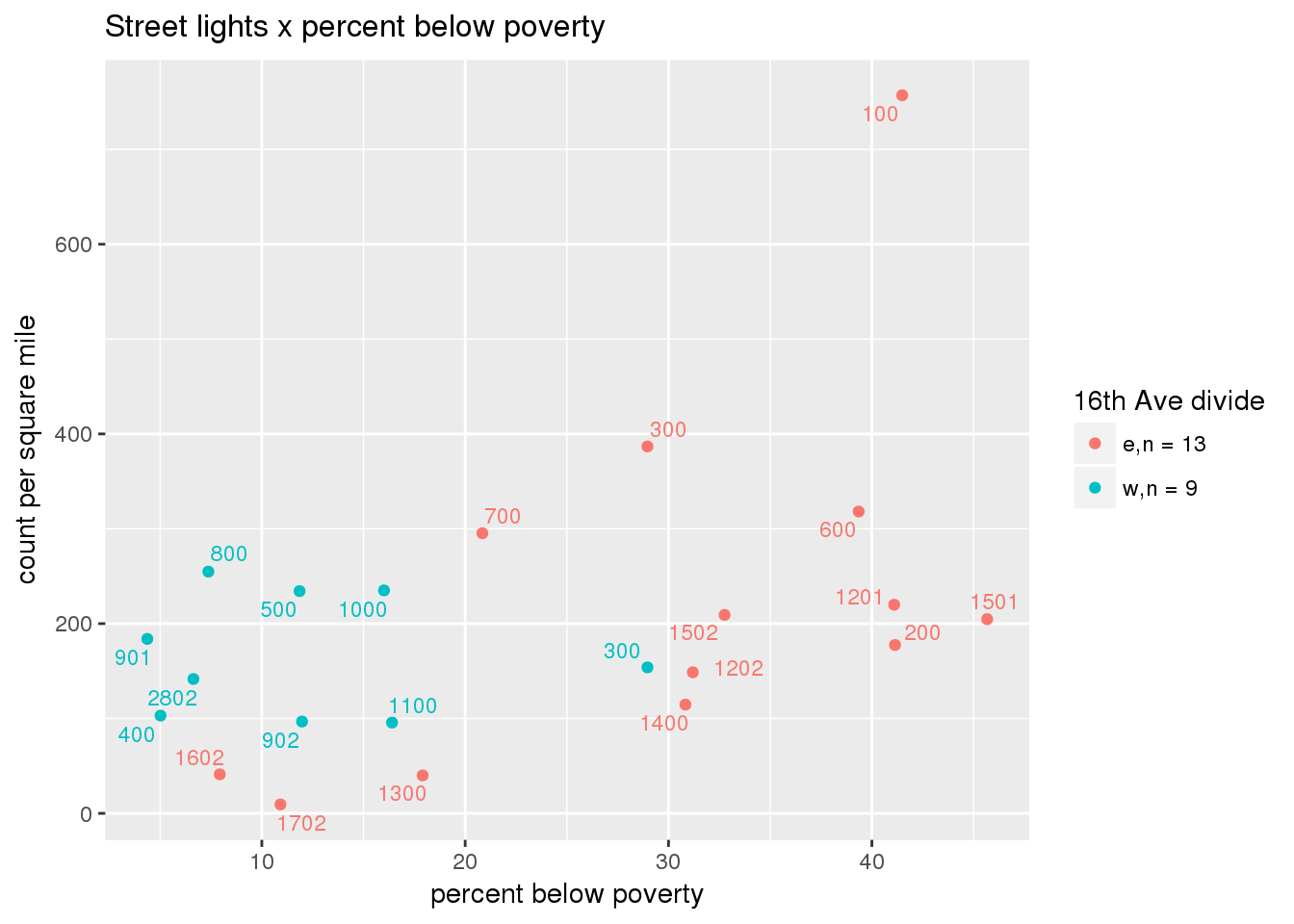
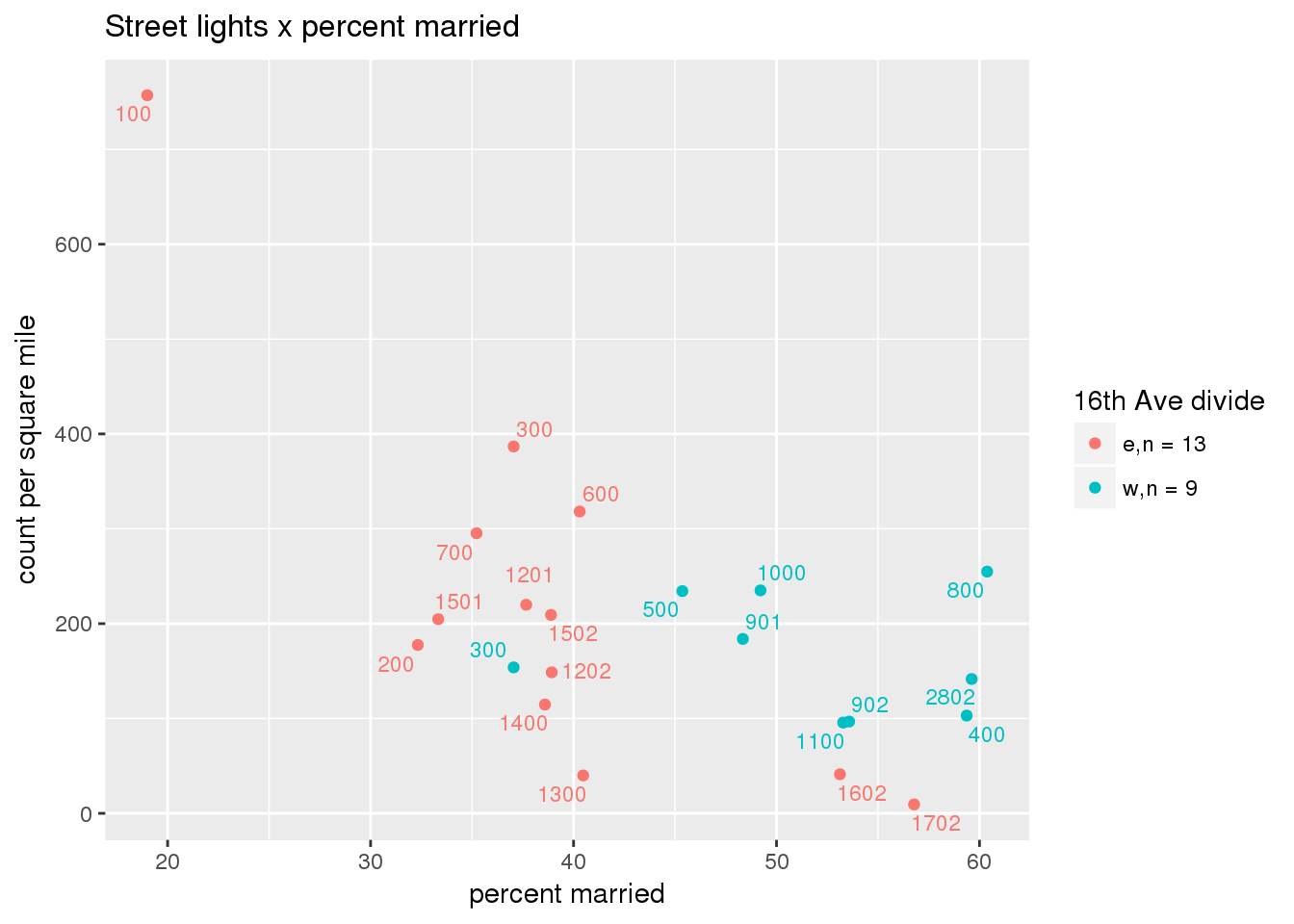
3.5.2 Street lights
Street lights
strtlights <- ptfcn(pttablename = "streetlights", normvar = "area", mytitle = "Street lights", legend_title = "16th Ave divide")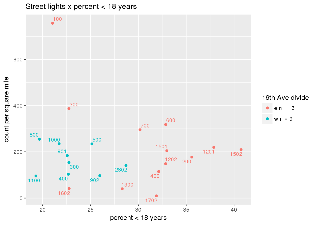
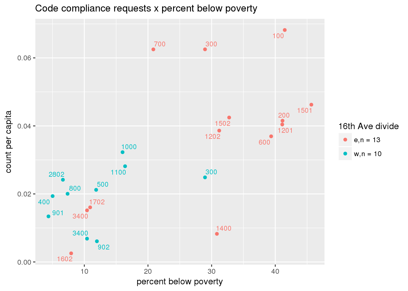
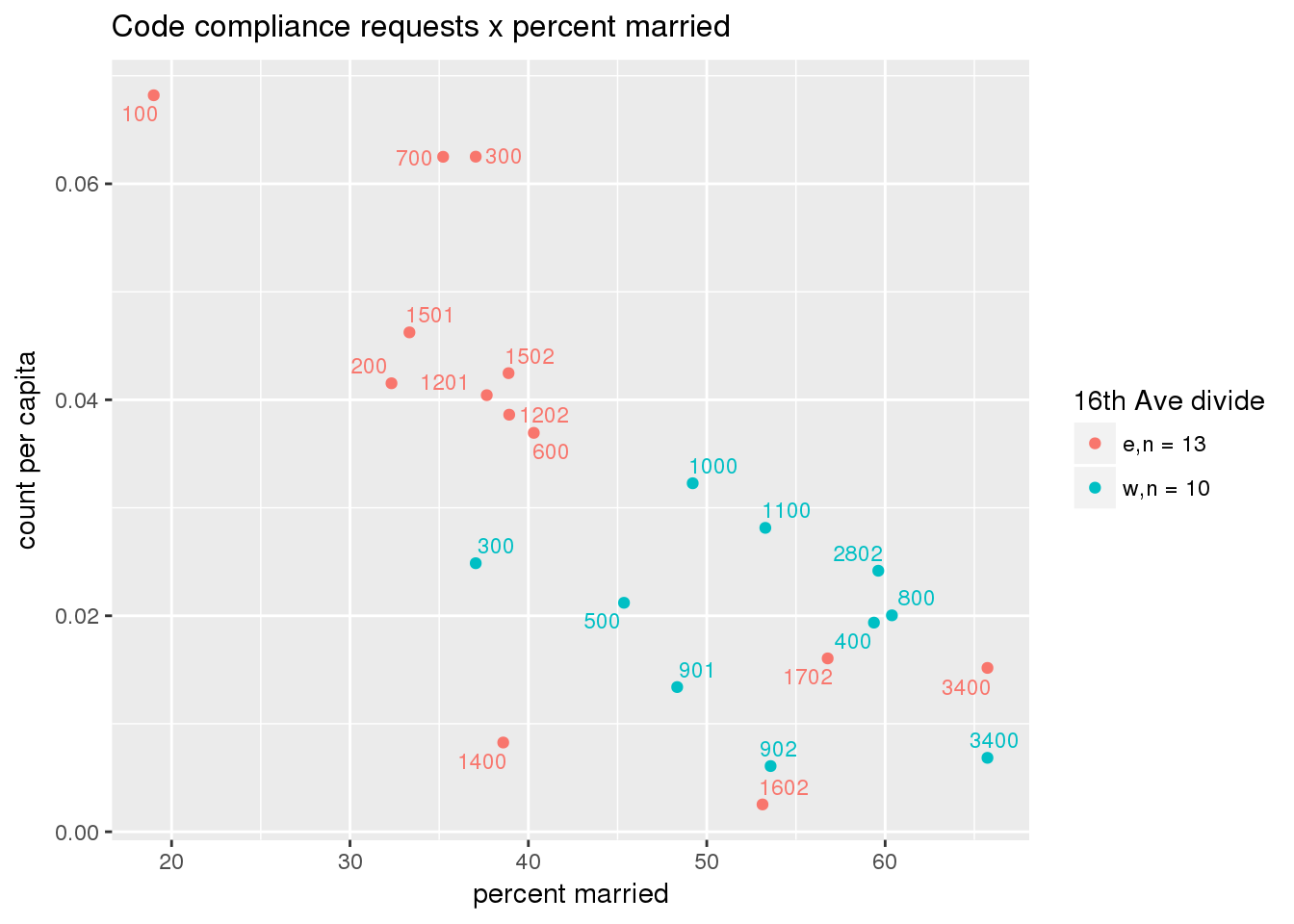
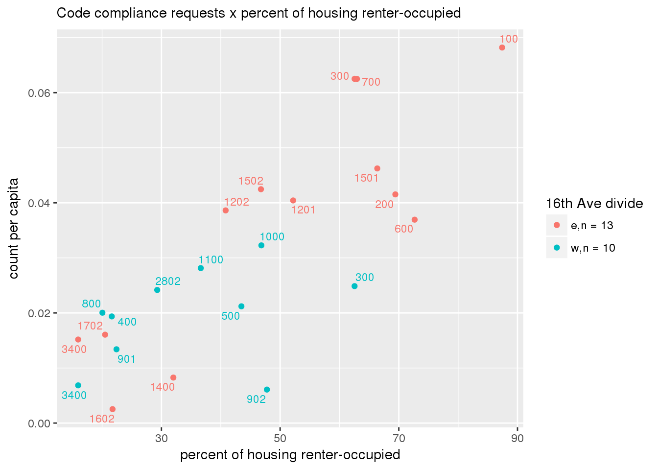
3.5.3 Code compliance requests
Counts of code compliance requests per capita
codecompliance <- ptfcn(pttablename = "codecompliance2015", normvar = "capita", mytitle = "Code compliance requests", legend_title = "16th Ave divide")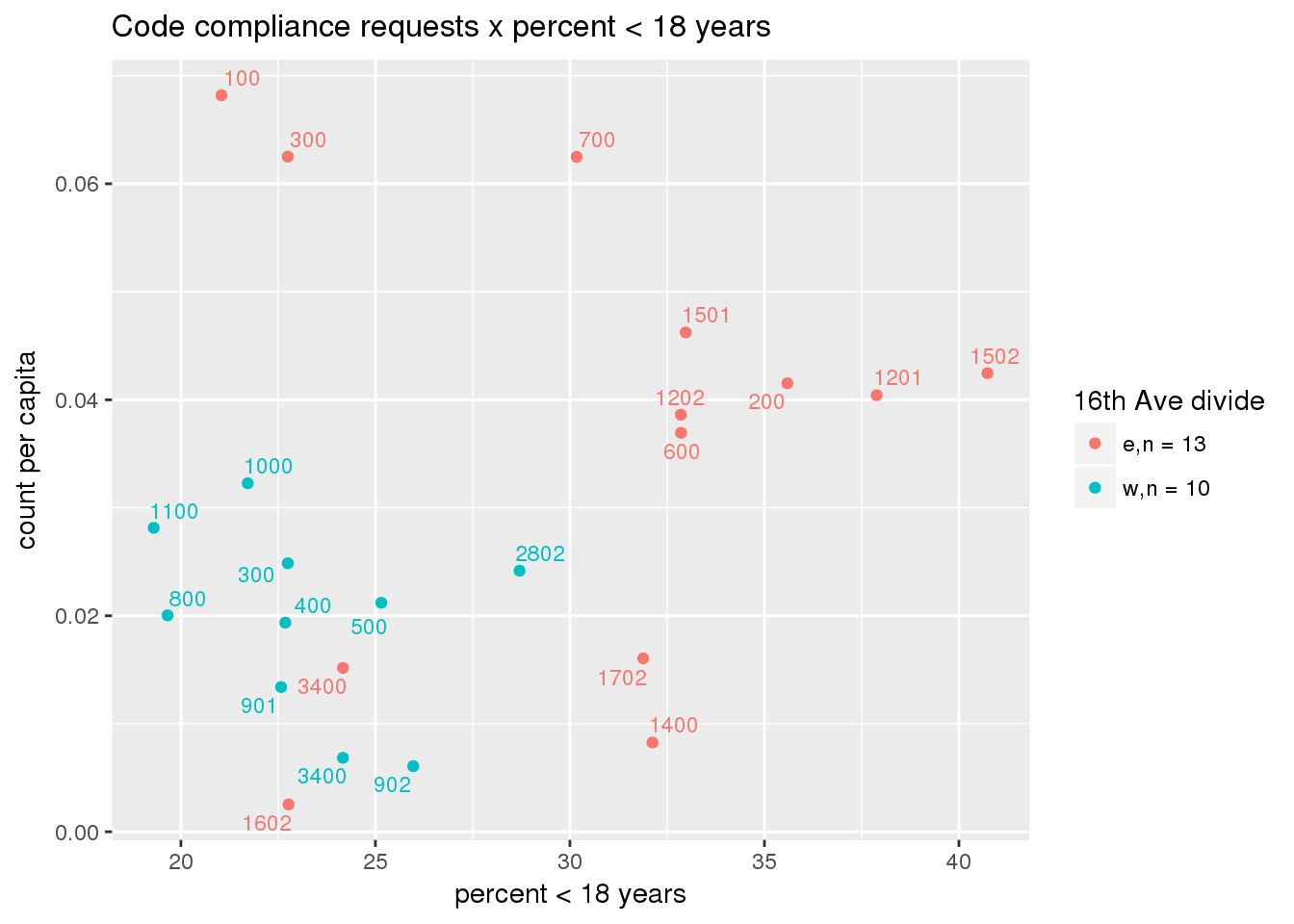
3.5.4 Transit
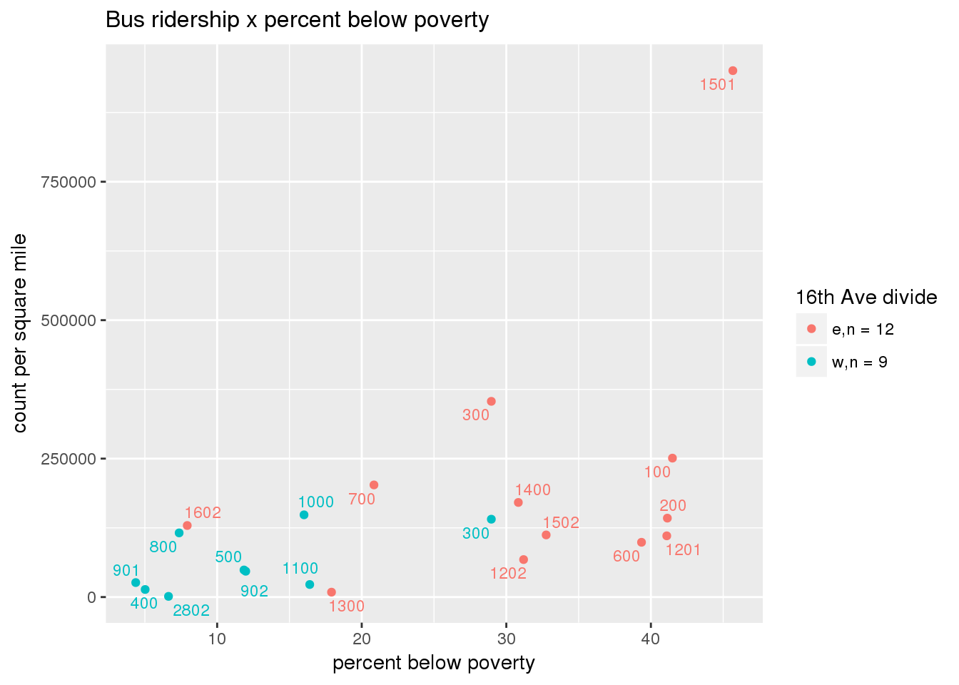
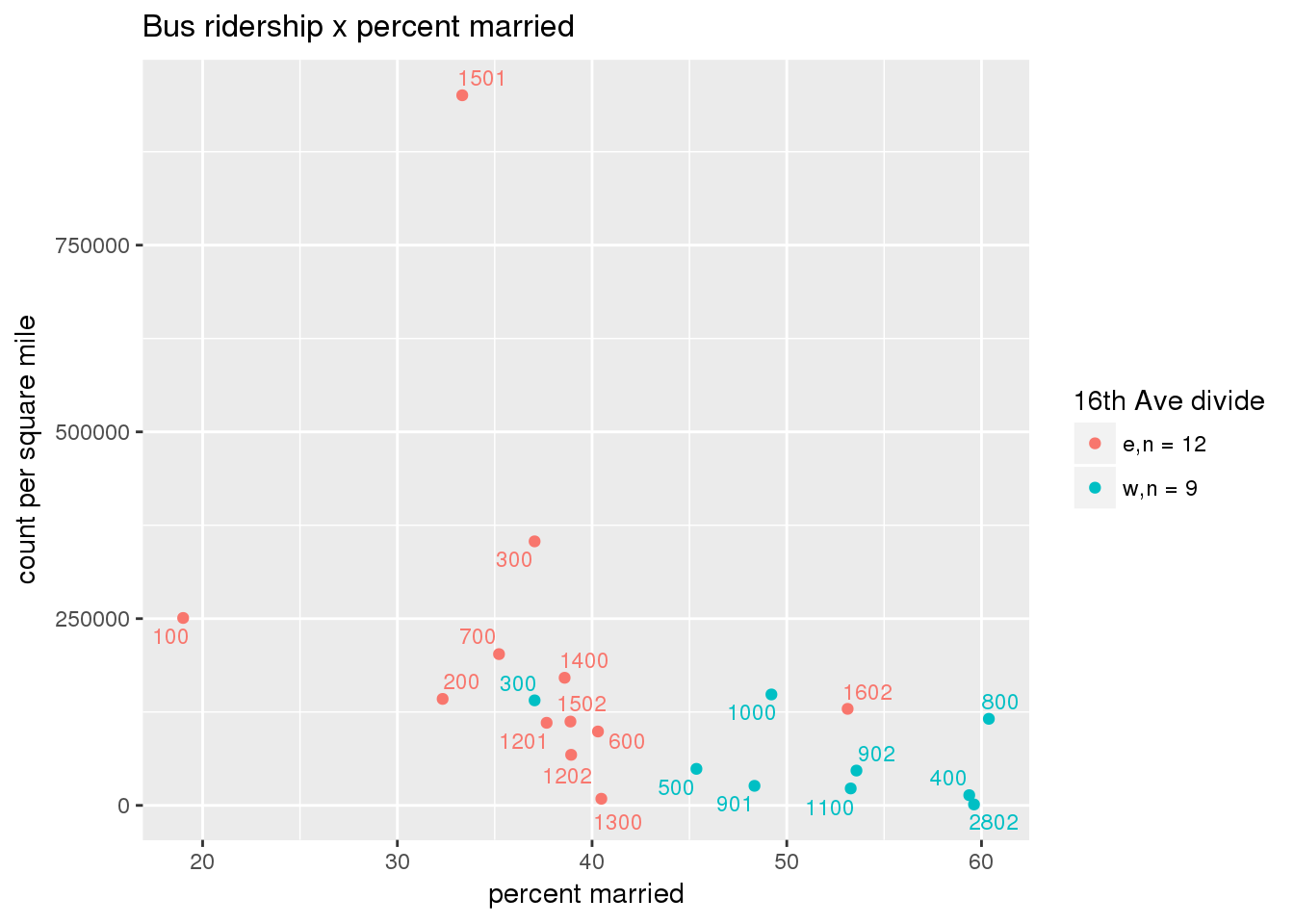
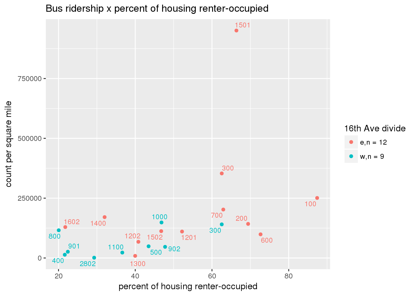
3.5.4.1 Ridership
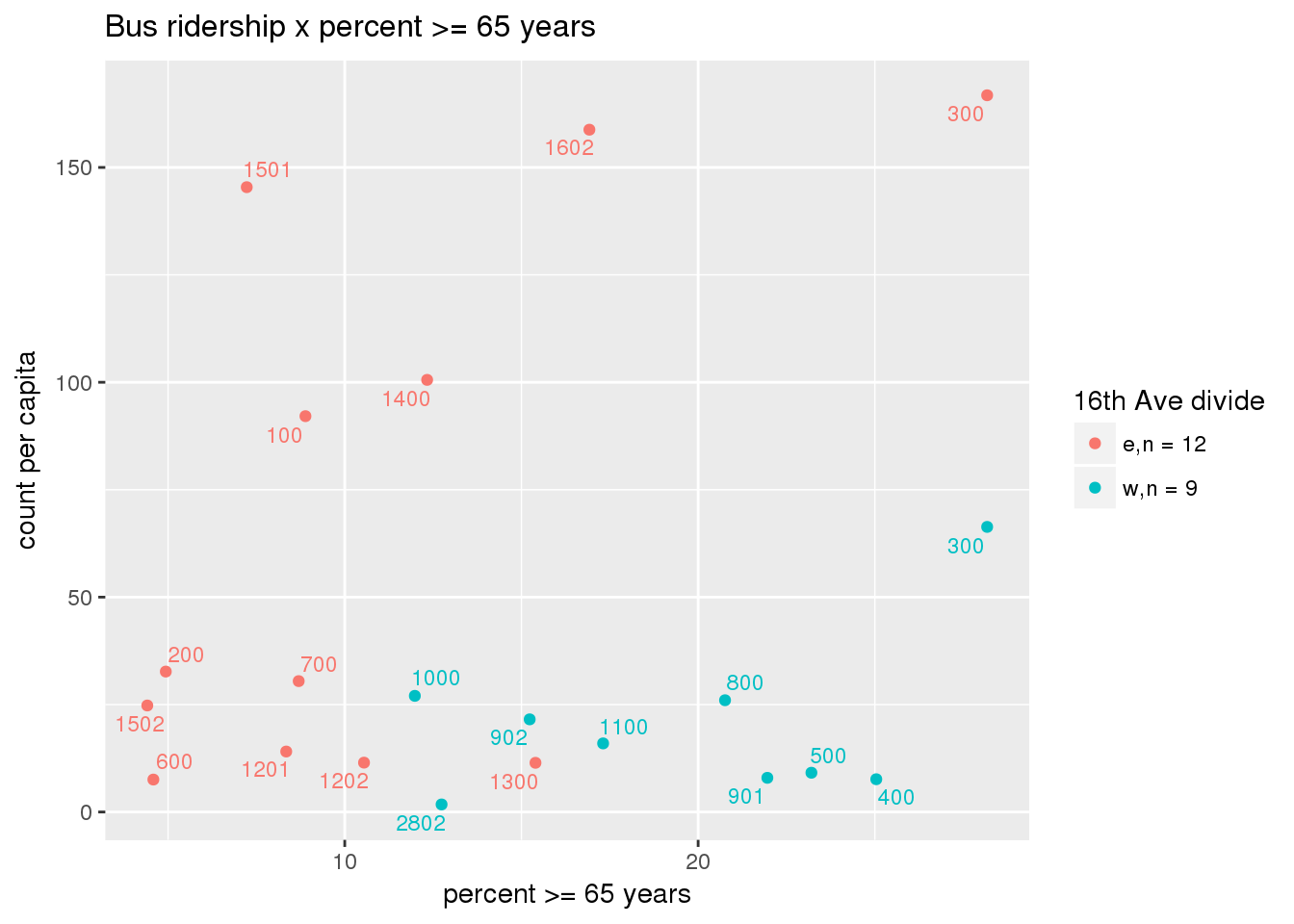
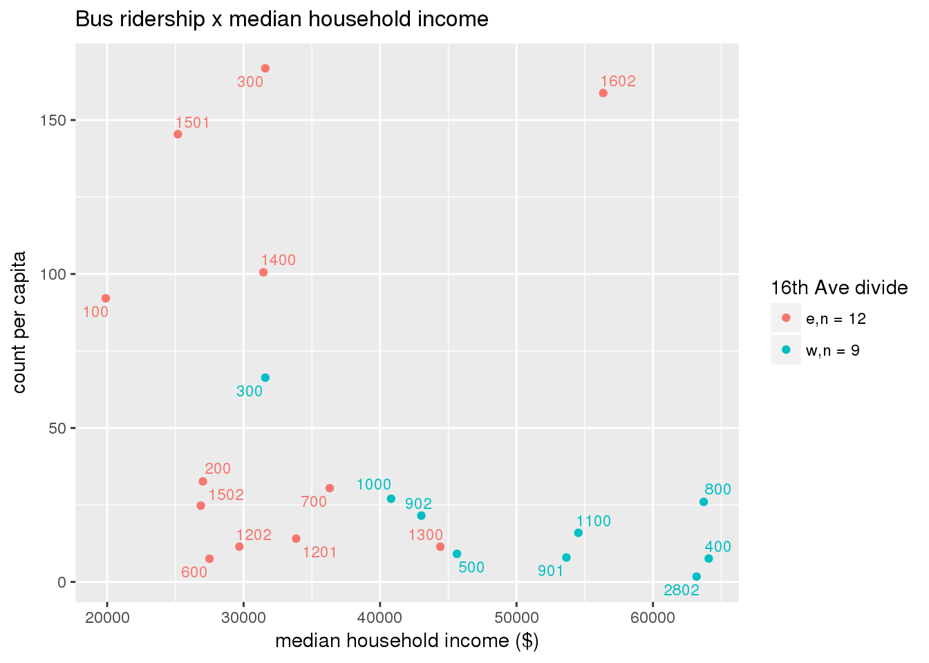
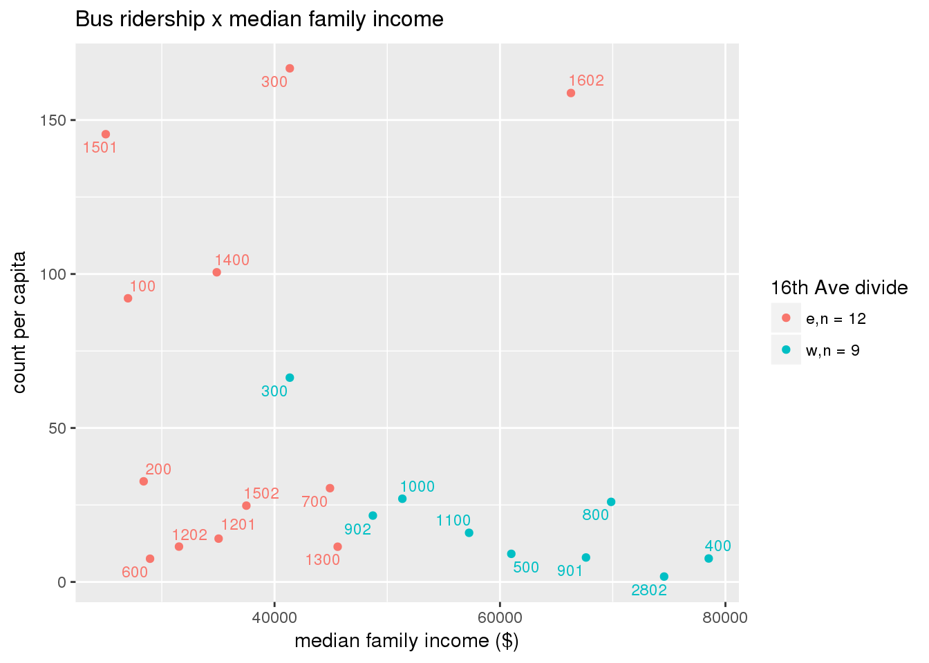
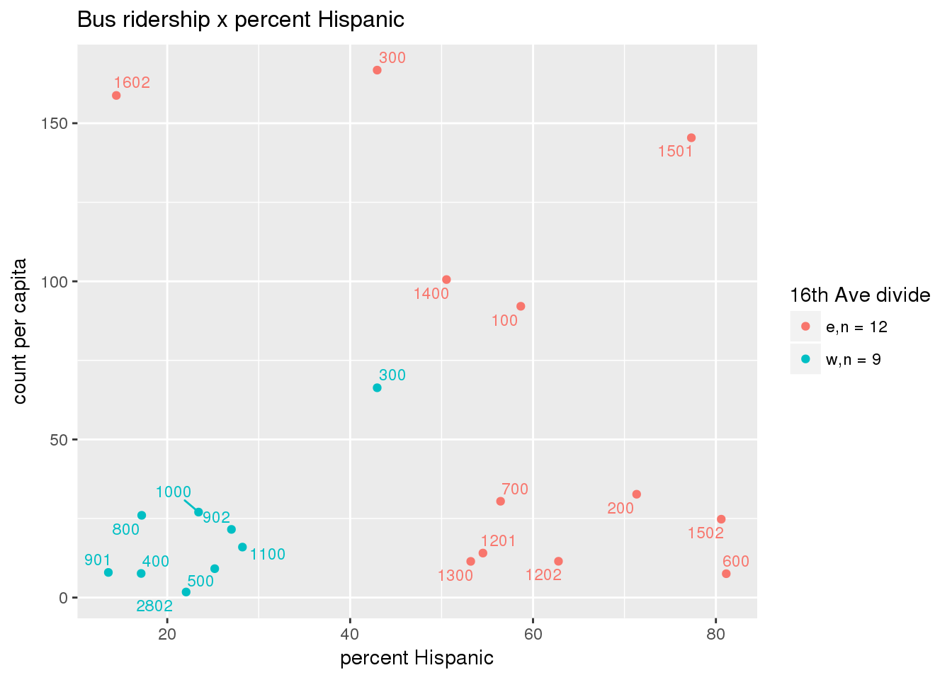
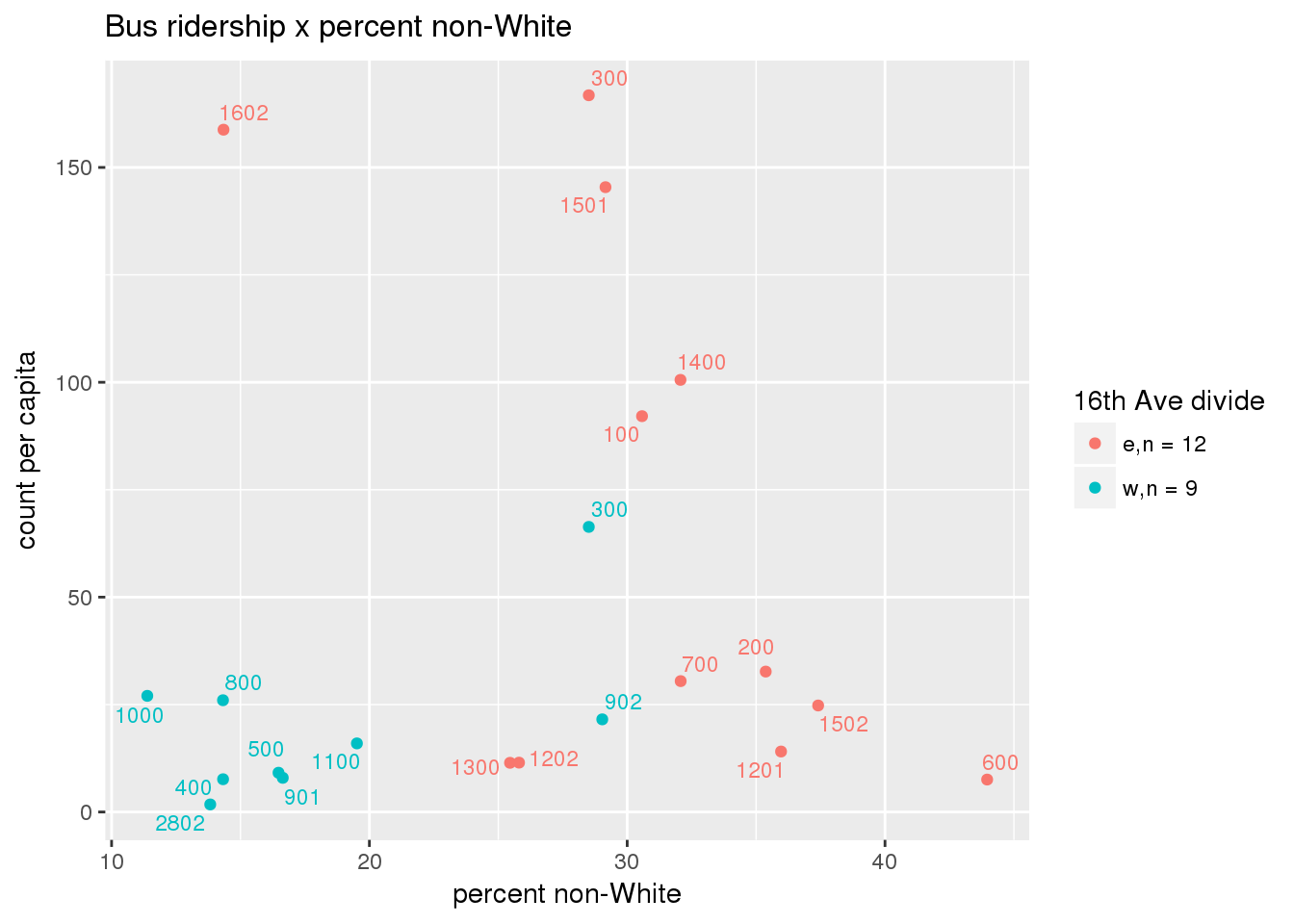
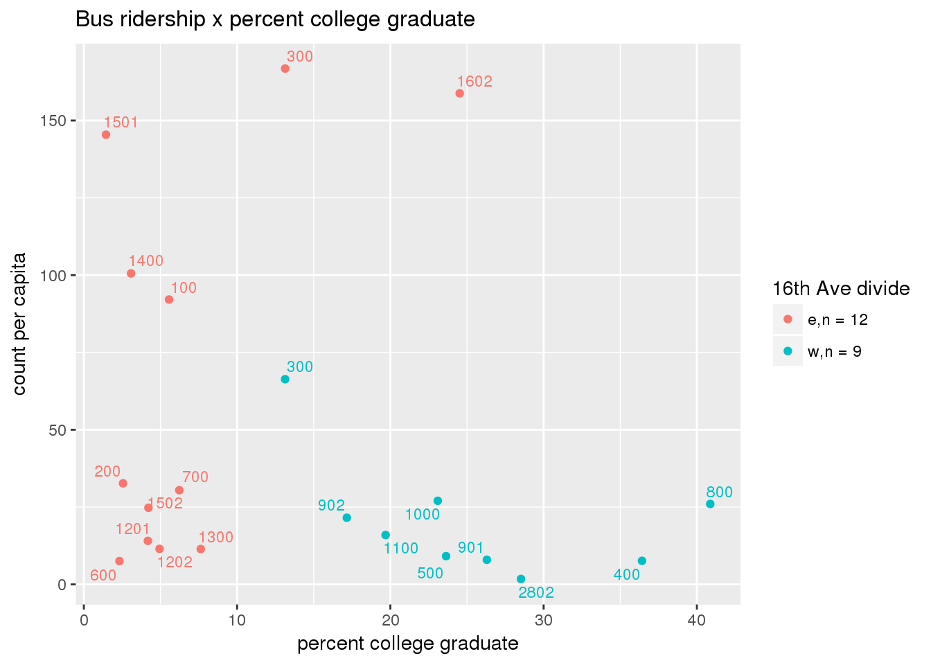
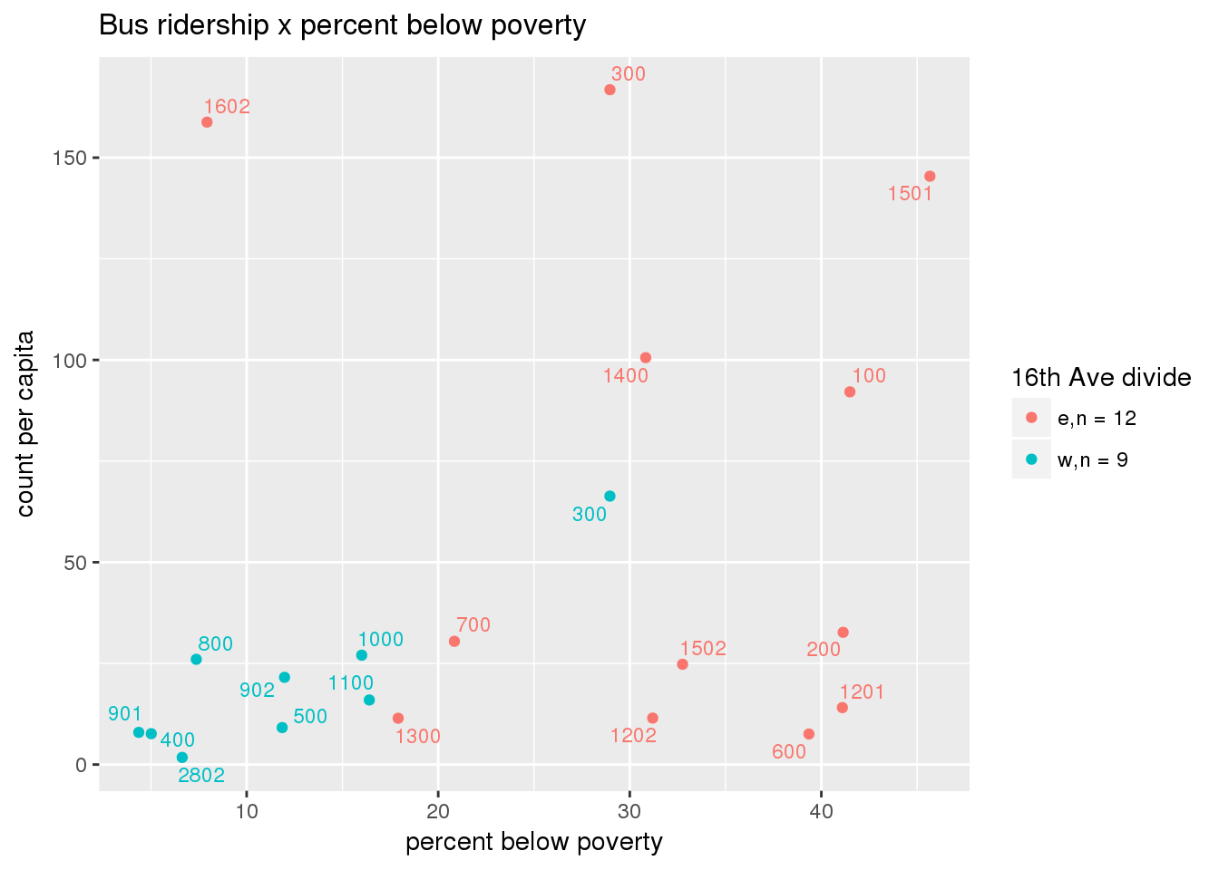
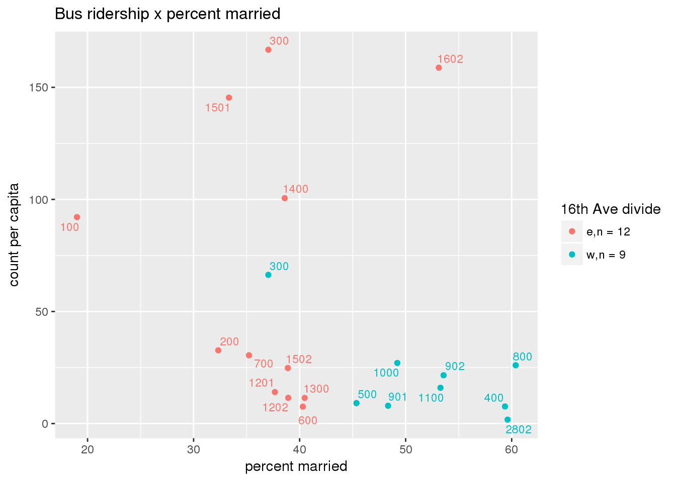
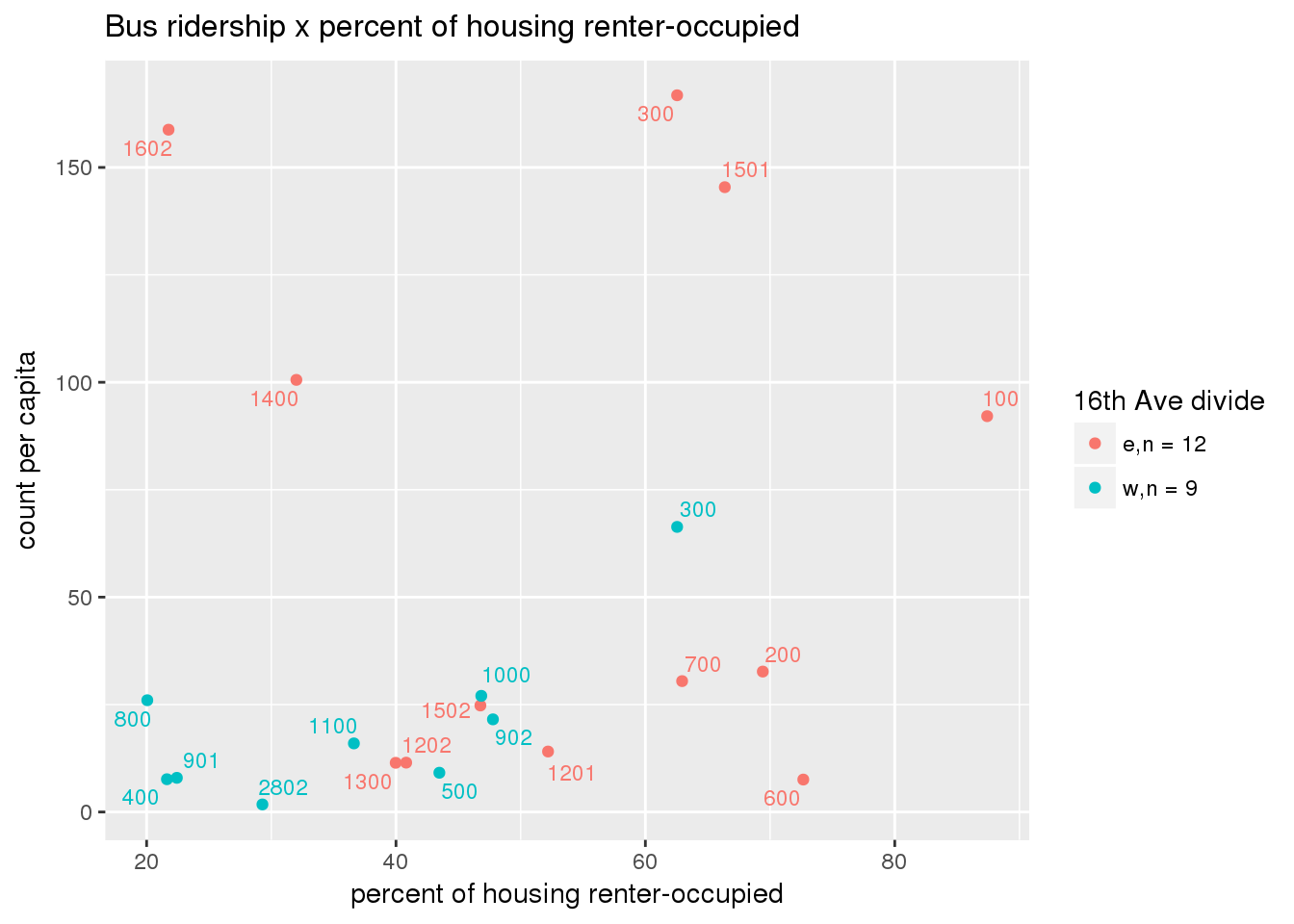
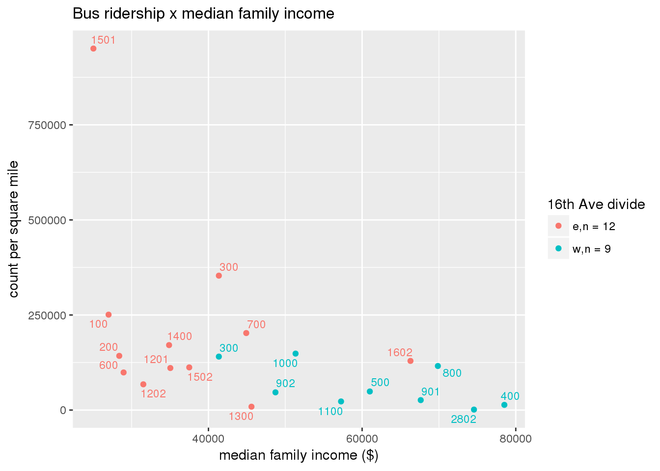
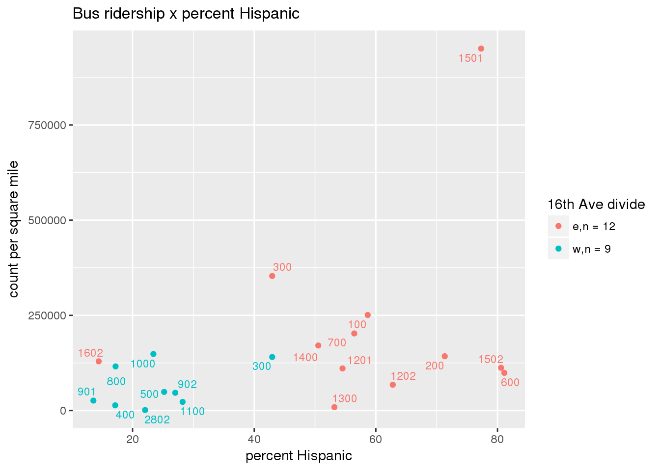
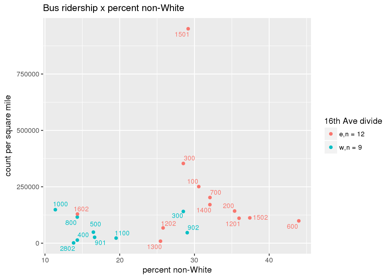
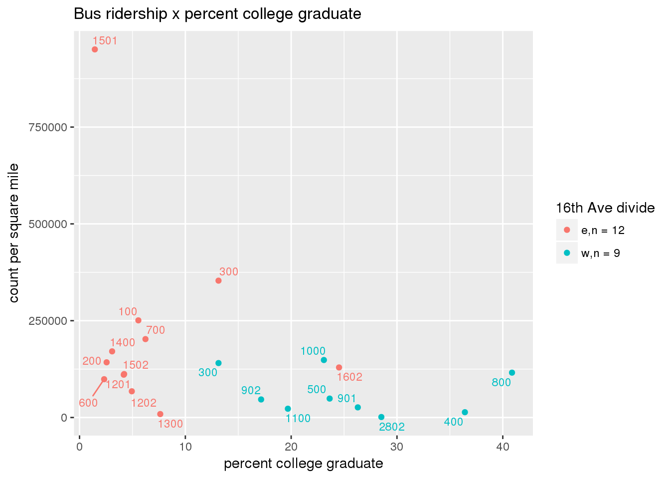
Bus ridership (summed alightings) per capita
riderfcn <- function(pttablename, where = "", normvar, mytitle){
rdsql <- "
with
--substitute input table and where clause
p as (select * from yakima_equity.ridershipstatistics)
--census tracts
, ct as (select st_area(the_geom_2286) as area_ct, * from yakima_equity.tract_2015)
--intersect points and tracts
, px as (select tract, zone_16th, alightings from ct, p where st_intersects(p.the_geom_2286, ct.the_geom_2286))
--jsum by tract
, pj as (select
--normalization
sum(alightings) / xxxNORMxxx as xxxNORMALIASxxx
, tract
, ct.zone_16th
from px left join ct using(tract)
group by tract, xxxNORMxxx
, ct.zone_16th
)
--join to tract data
, f as (select pj.*
, median_hh_income
, median_family_income
, age_lt_18 / total_pop::numeric * 100 as pct_age_lt_18
, age_ge_65 / total_pop::numeric * 100 as pct_age_ge_65
, eth_hispanic / total_pop::numeric * 100 as pct_hispanic
, race_nonwhite / total_pop::numeric * 100 as pct_nonwhite
, case when (edu_collgrad + edu_9th_somecoll + edu_lt_9th) = 0 then 0 else edu_collgrad::numeric / (edu_collgrad + edu_9th_somecoll + edu_lt_9th) * 100 end as pct_collgrad
, case when pov_status = 0 then 0 else pov_below_100pct / pov_status::numeric * 100 end as pct_below_poverty
, case when married + unmarried = 0 then 0 else married / (married + unmarried)::numeric * 100 end as pct_married
, case when housingunits_renter + housingunits_owner = 0 then 0 else housingunits_renter / (housingunits_renter + housingunits_owner)::numeric * 100 end as pct_renter from pj join ct using(tract, zone_16th))
select * from f;
"
yvar <- switch(normvar,
capita = "count_per_capita",
area = "count_per_mi2")
ylab <- switch(normvar,
capita = "count per capita",
area = "count per square mile")
normfield <- switch(normvar,
capita = "total_pop",
area = "(area_ct / 5280^2)")
normalias <- switch(normvar,
capita = "count_per_capita",
area = "count_per_mi2")
mySql <- gsub("xxxPTDATAxxx", pttablename, gsub("xxxNORMxxx", normfield, gsub("xxxNORMALIASxxx", normalias, gsub("xxxWHERExxx", where, rdsql))))
assign("mySQL", mySql, envir = .GlobalEnv)
dat <- dbGetQuery(conn = dbconn, statement = mySql)
# plot
xvars <- list(
c('pct_age_lt_18', 'percent < 18 years'),
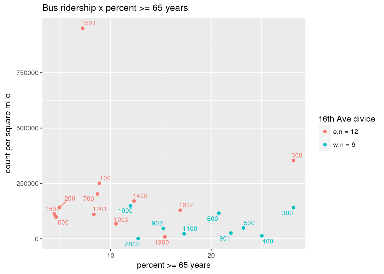
c('pct_age_ge_65', 'percent >= 65 years'),
c('median_hh_income', 'median household income'),
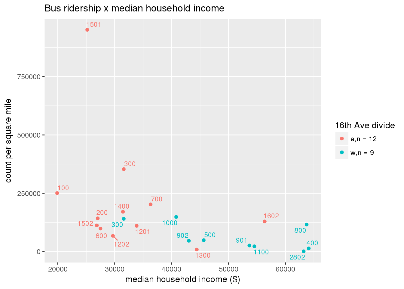
c('median_family_income', 'median family income'),
c('pct_hispanic', 'percent Hispanic'),
c('pct_nonwhite', 'percent non-White'),
c('pct_collgrad', 'percent college graduate'),
c('pct_below_poverty', 'percent below poverty'),
c('pct_married', 'percent married'),
c('pct_renter', 'percent of housing renter-occupied'))
for(i in xvars){
#message(i)
thetitle <- sprintf("%s x %s", mytitle, i[2])
xlab <- gsub("income", "income ($)", gsub("pct_", "percent", i[2]))
g <- corplotgg_fill(dat = dat, xvar = i[1], yvar = yvar, fillvar = "zone_16th", mytitle = thetitle, xlab = xlab, ylab = ylab, legend_title = "16th Ave divide")
print(g)
imgfile <- tolower(gsub("x_", "", gsub("_+", "_", gsub(" |[[:punct:]]", "_", thetitle))))
ggsave(filename = file.path(imagedir, sprintf("%s.png", imgfile)), plot = g, width = ggsavewidth, height = ggsaveheight, units = "in")
}
}
riderfcn(pttablename = "ridershipstatistics", normvar = "capita", mytitle = "Bus ridership")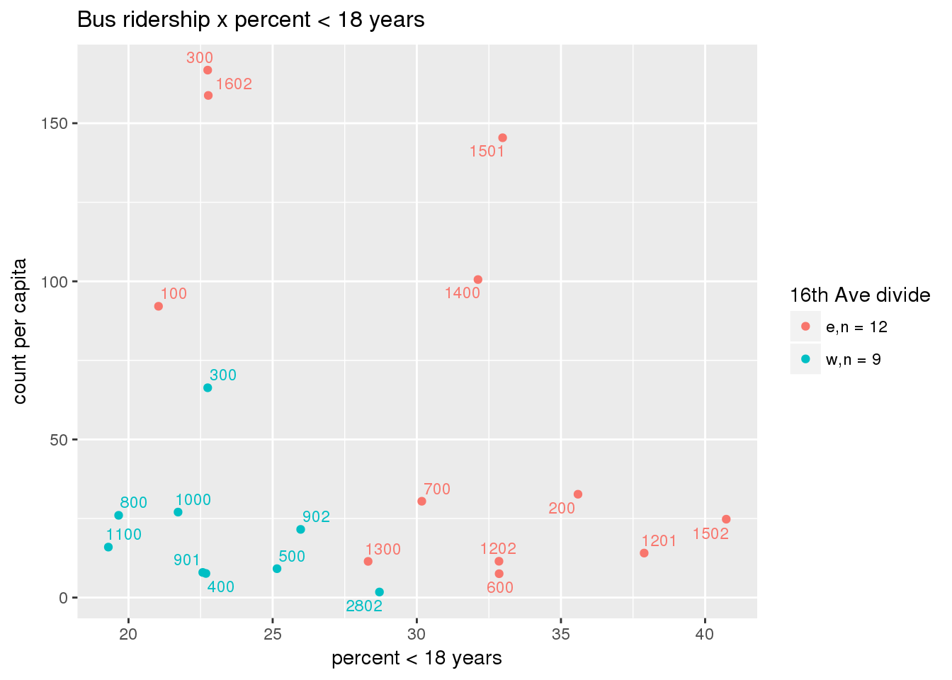
Bus ridership normalized by area:
riderfcn(pttablename = "ridershipstatistics", normvar = "area", mytitle = "Bus ridership")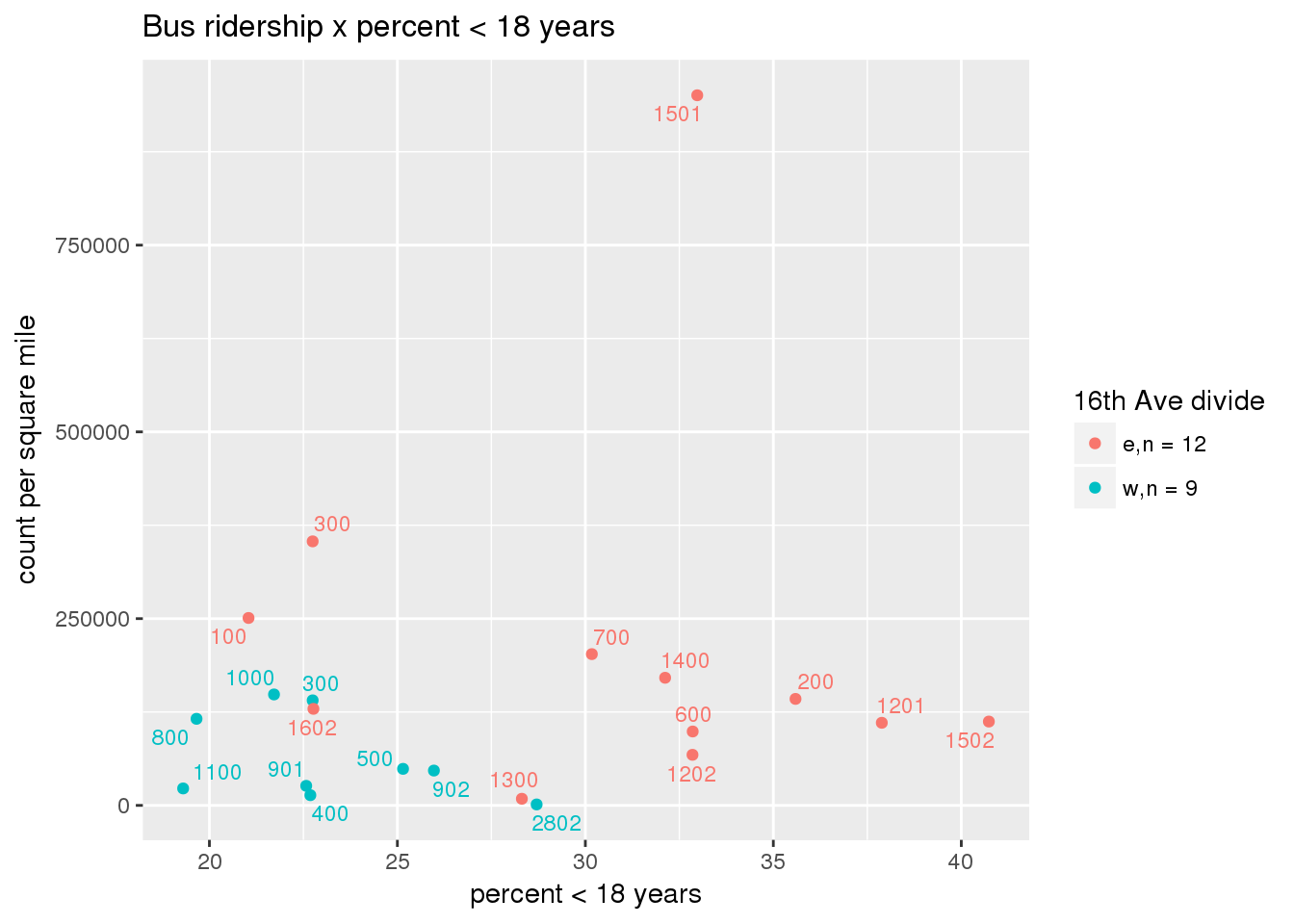
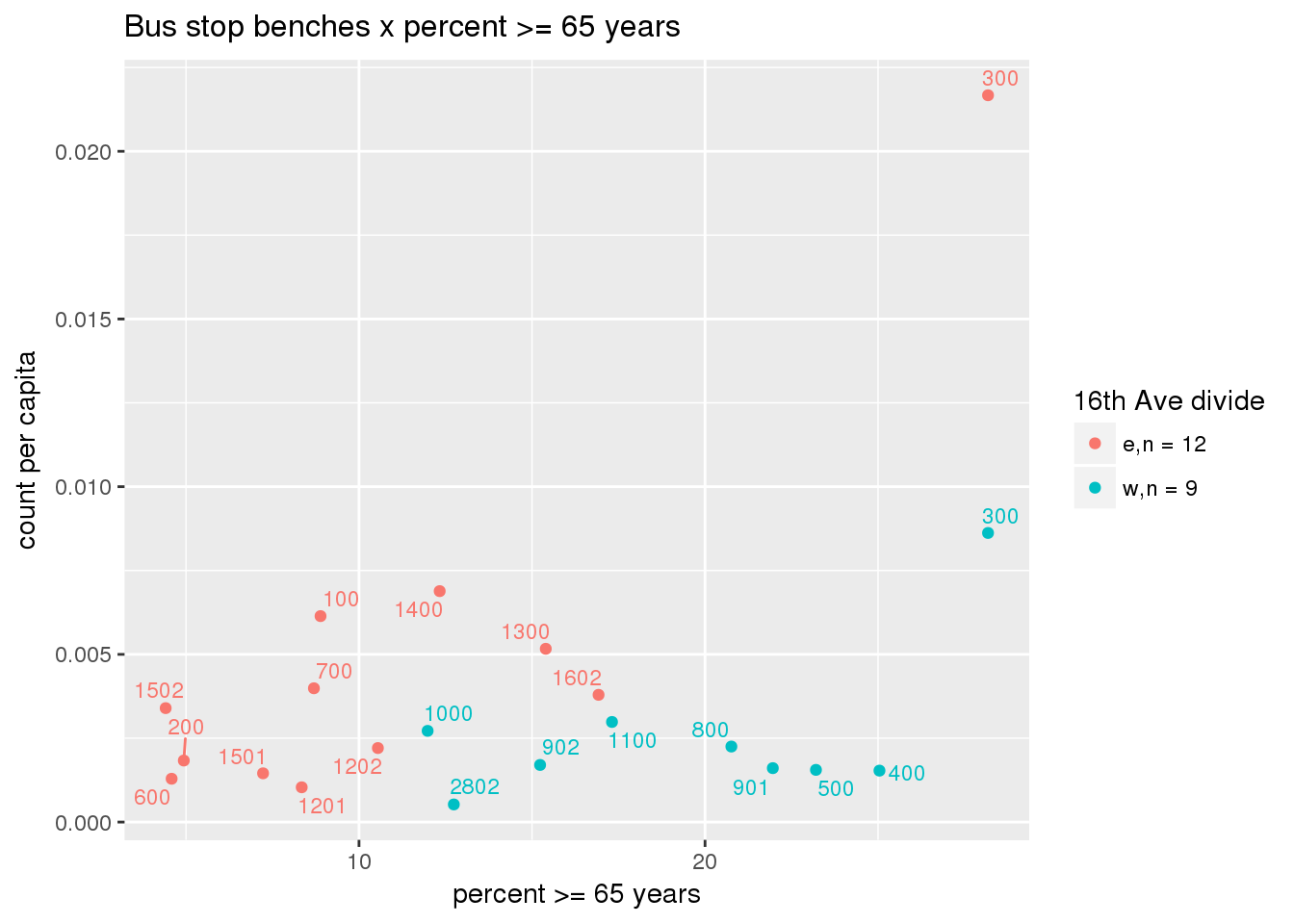
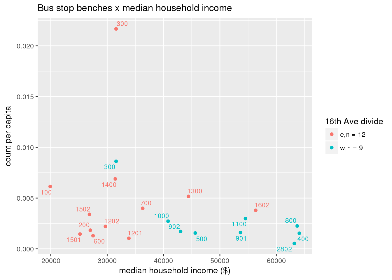
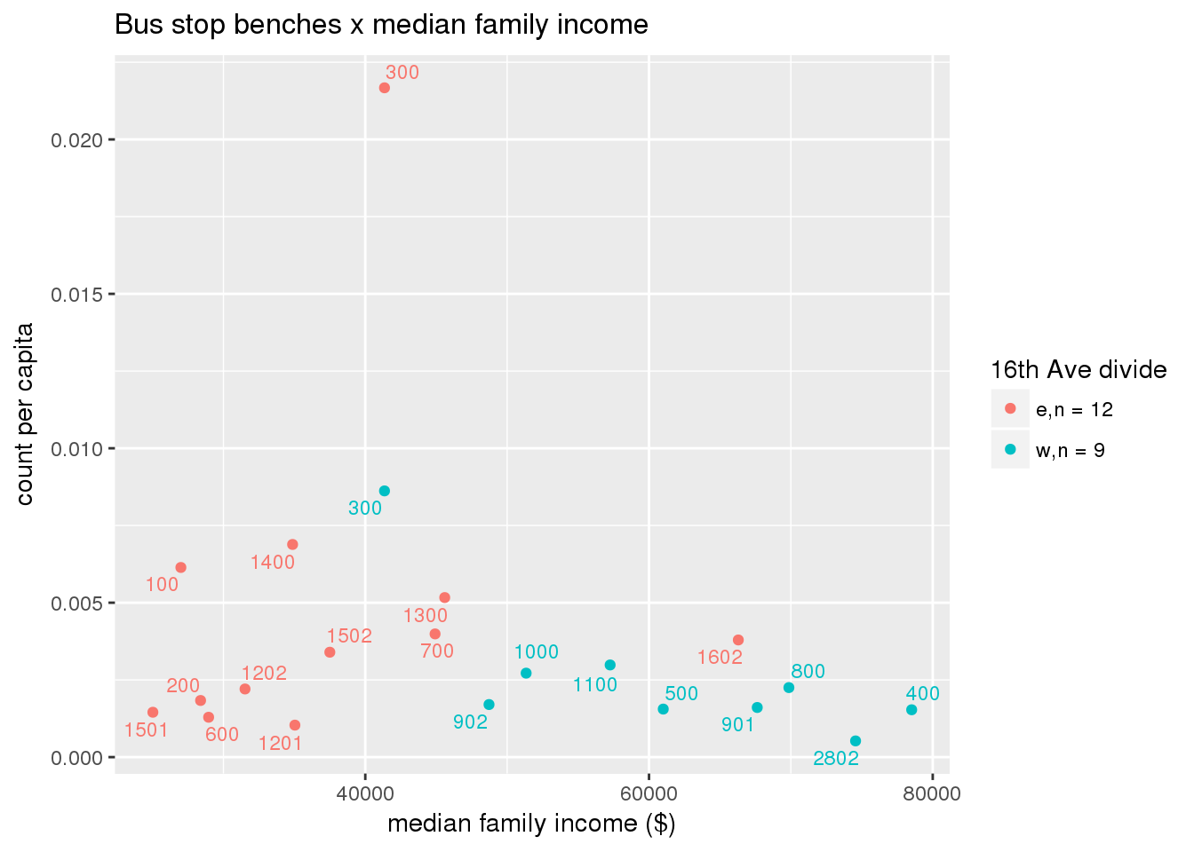
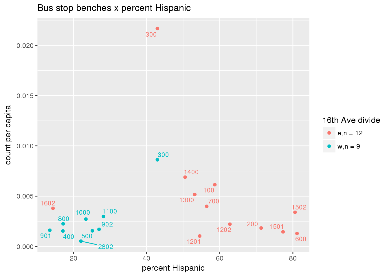
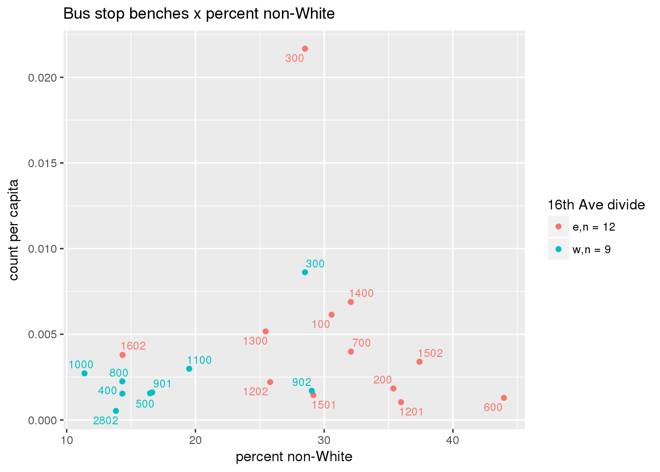
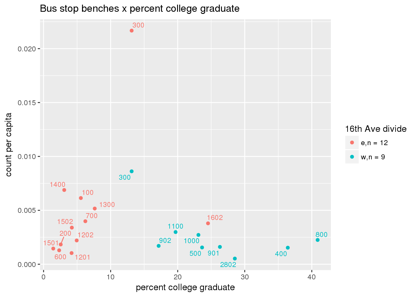
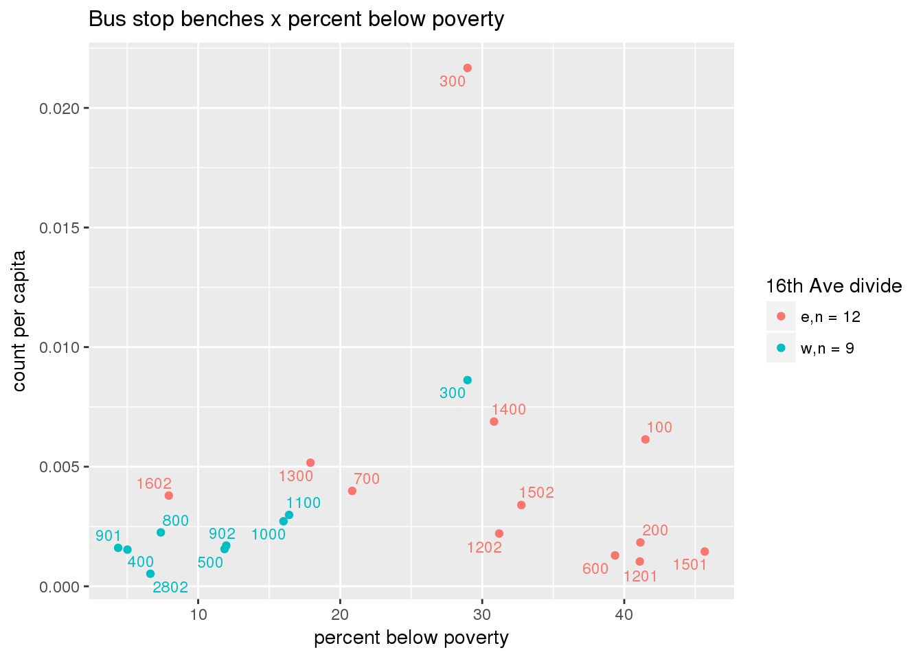
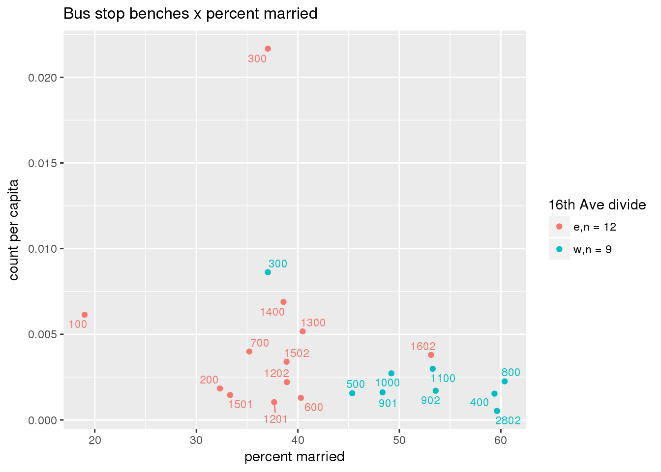
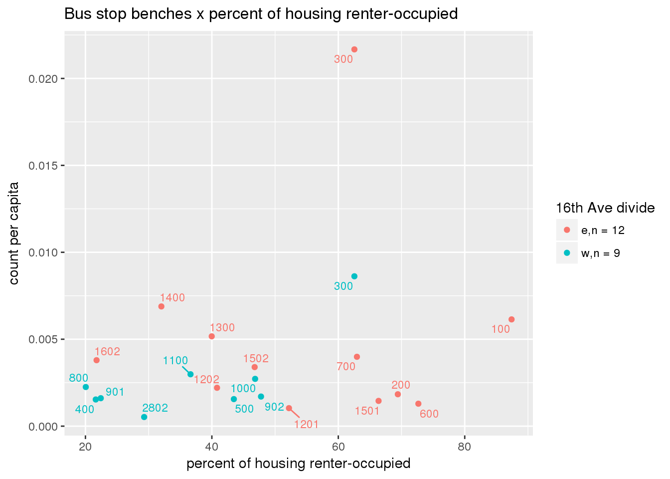
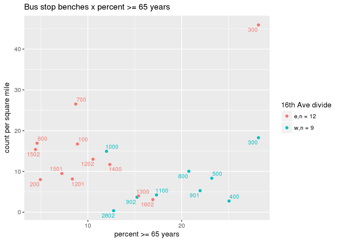
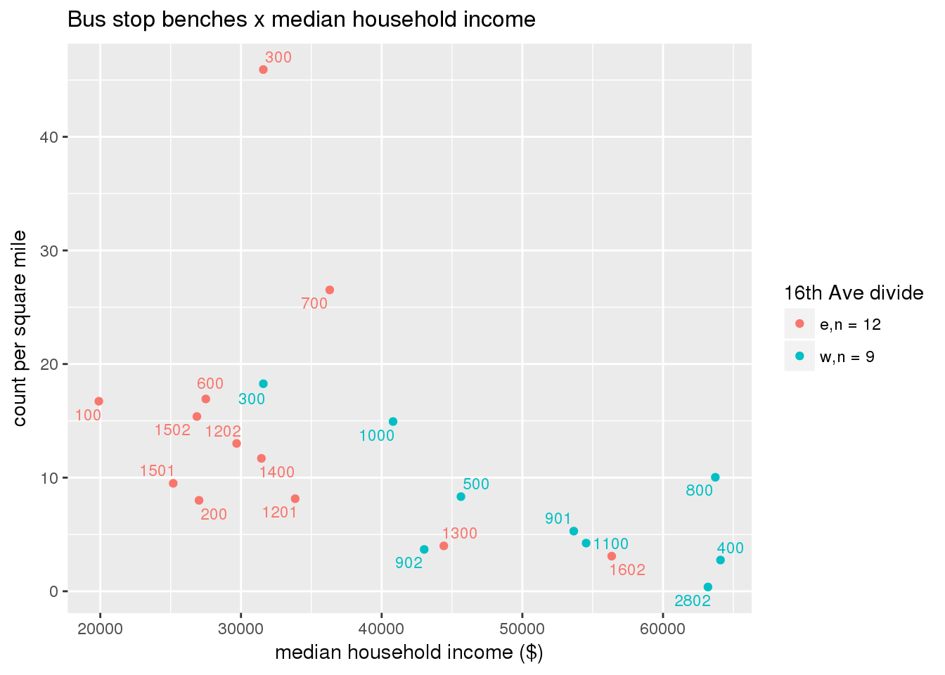
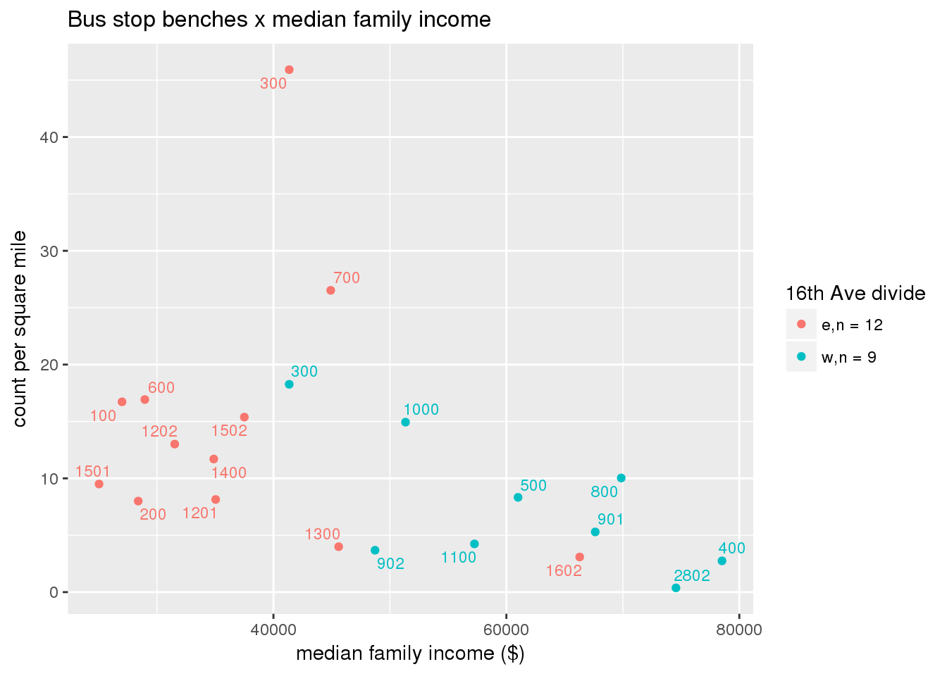
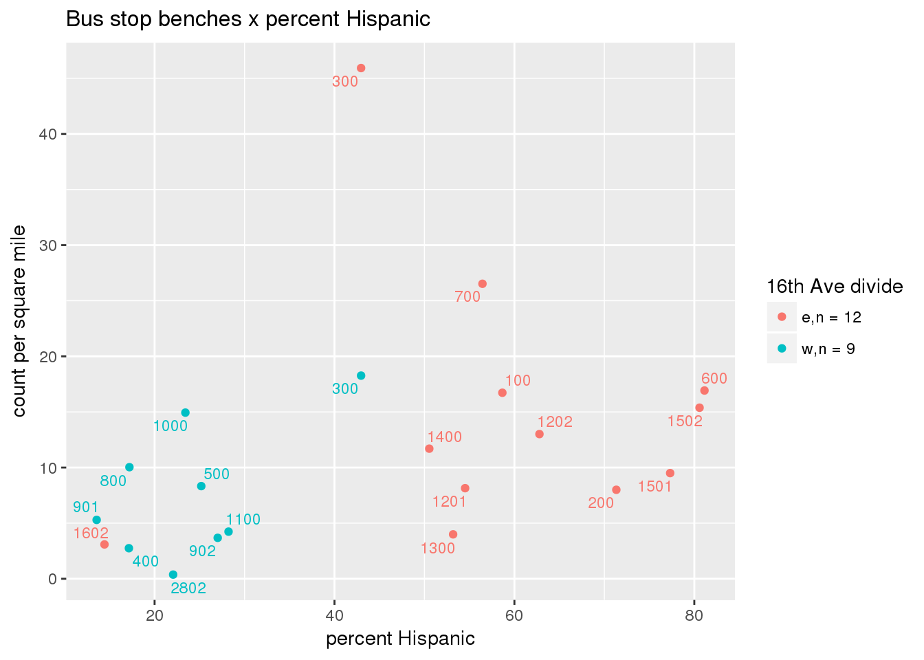
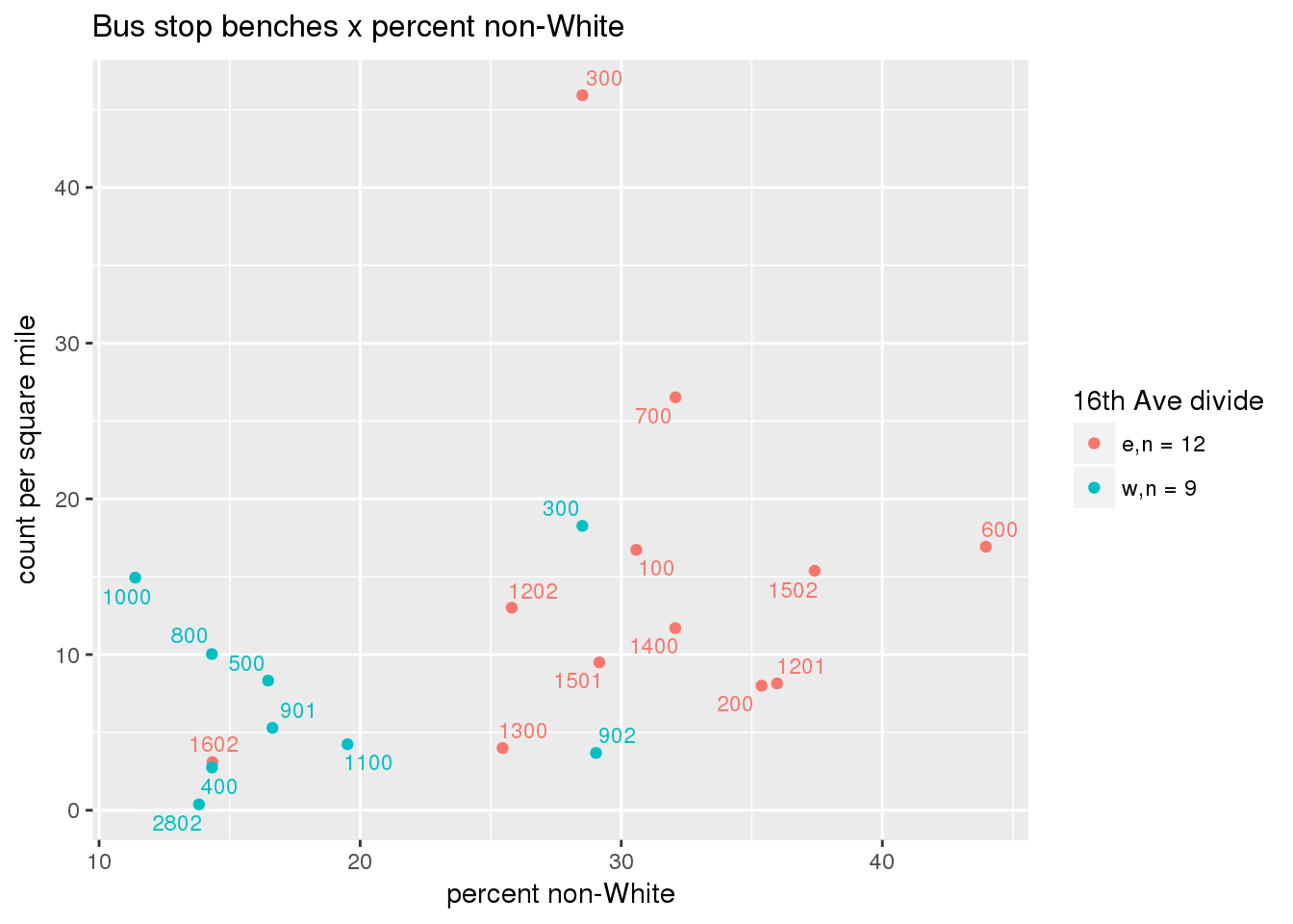
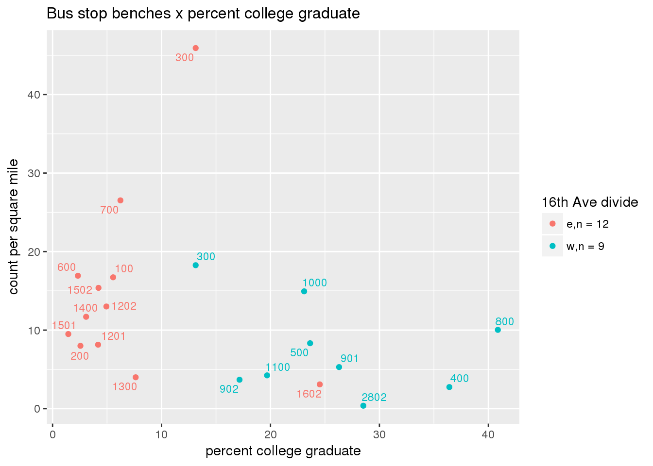
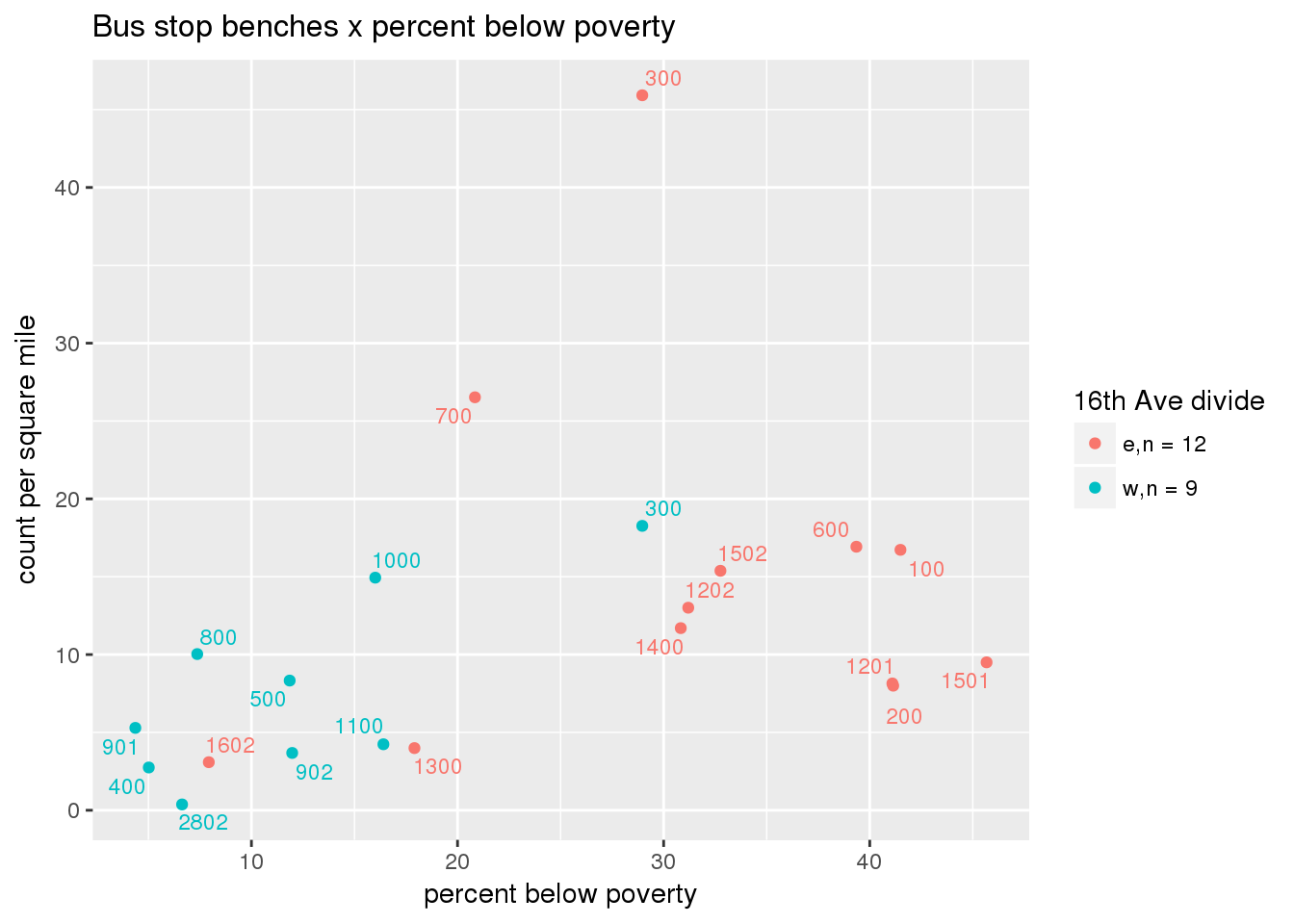
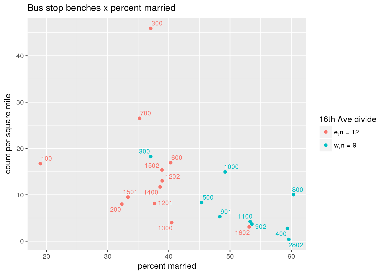
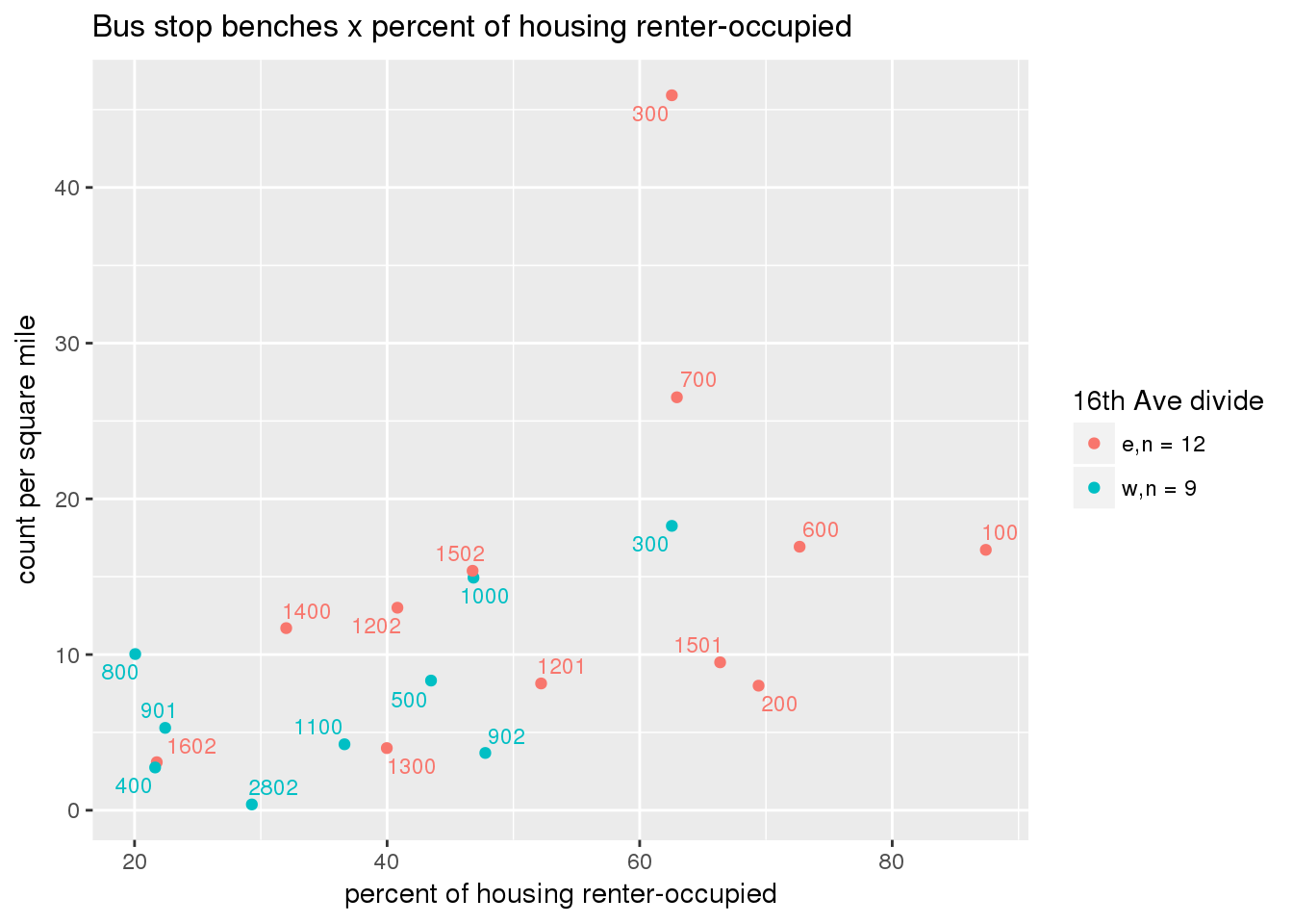
3.5.4.2 Benches
Bus benches per capita
busbenches <- ptfcn(pttablename = "busstops", where = "where bench = 'Y'", normvar = "capita", mytitle = "Bus stop benches", legend_title = "16th Ave divide")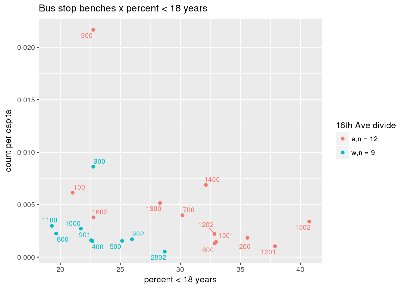
Bus benches normalized by area
busbench_norm <- ptfcn(pttablename = "busstops", where = "where bench = 'Y'", normvar = "area", mytitle = "Bus stop benches", legend_title = "16th Ave divide")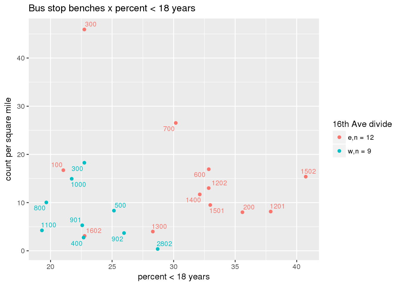
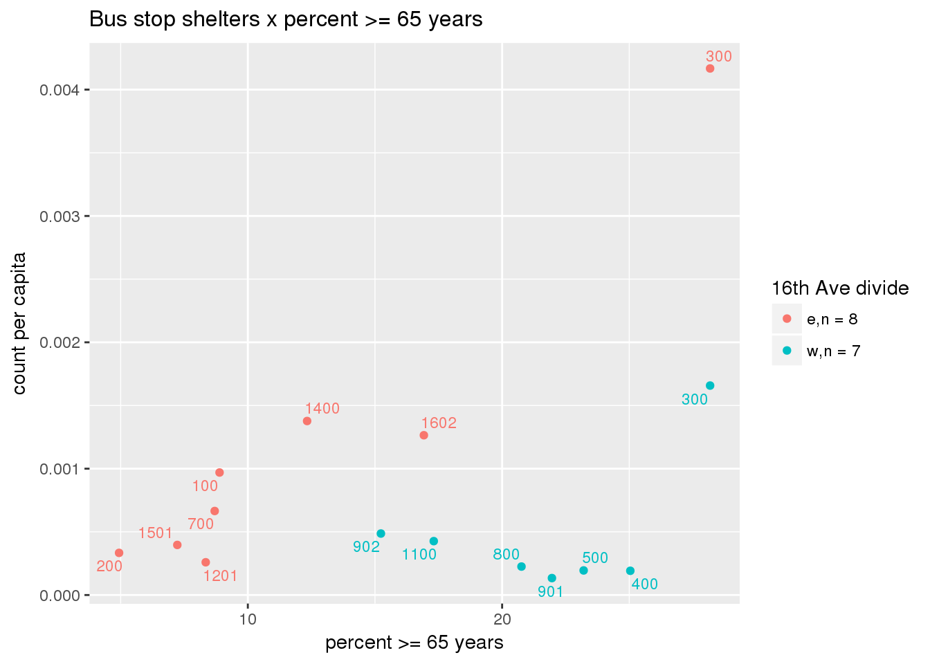
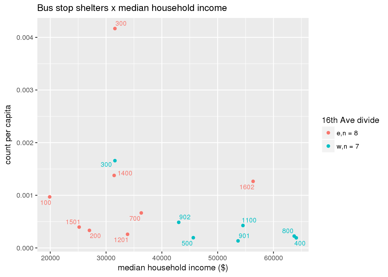
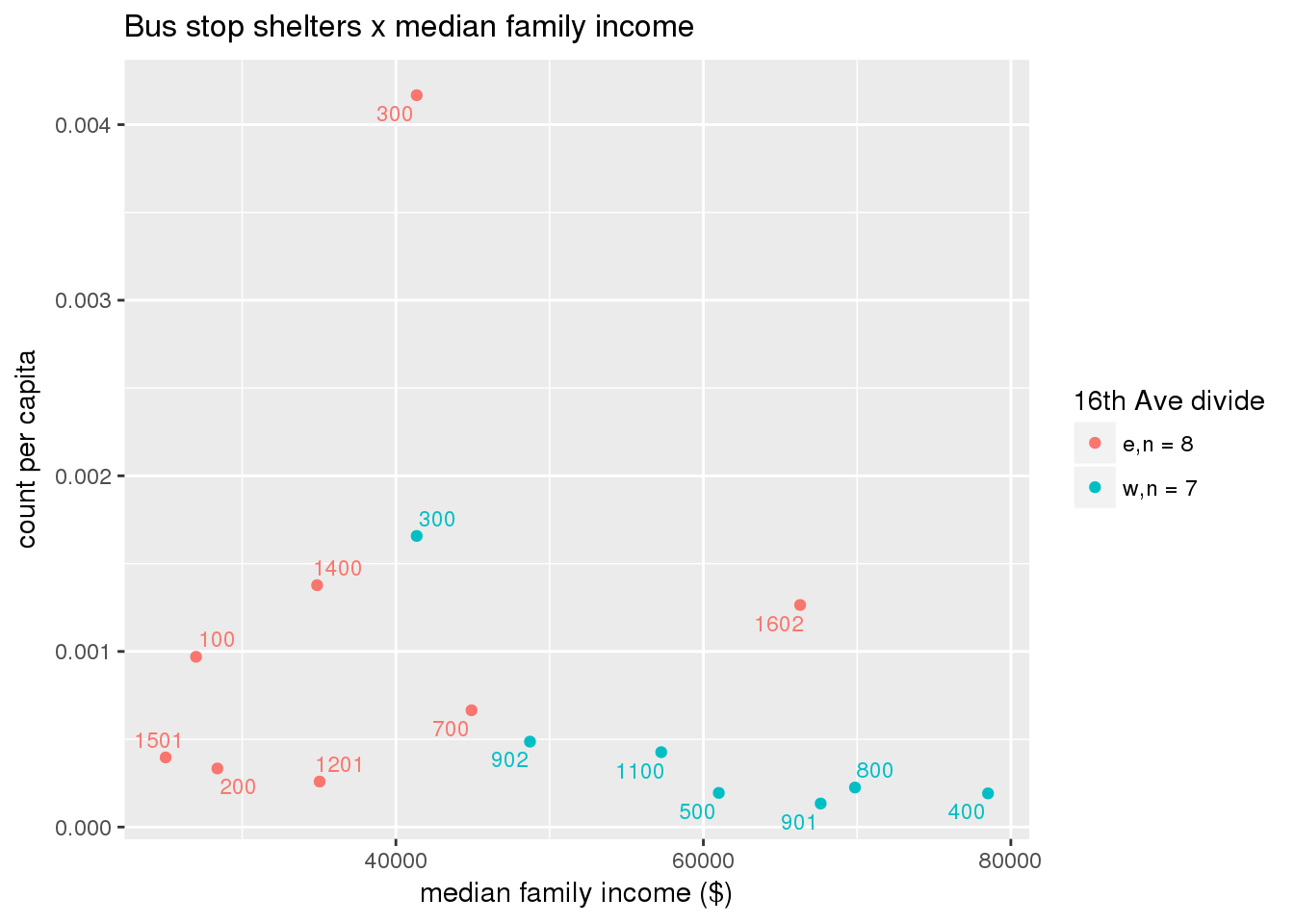
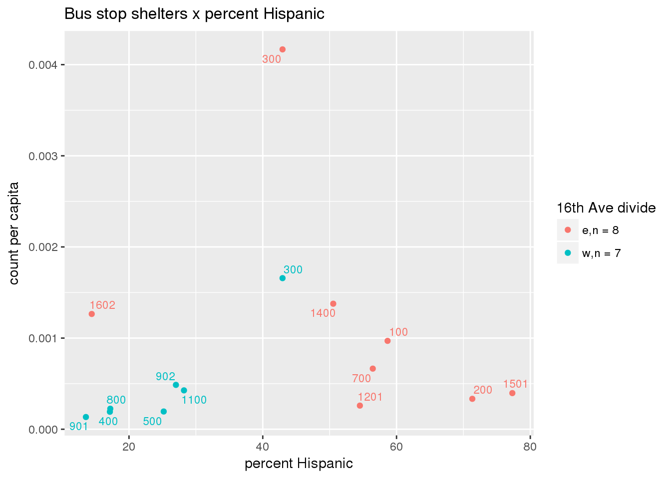
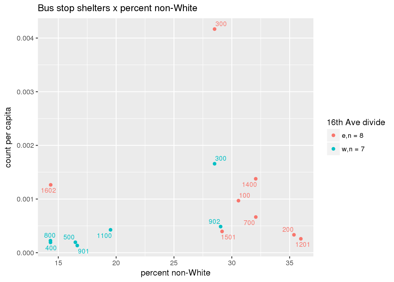
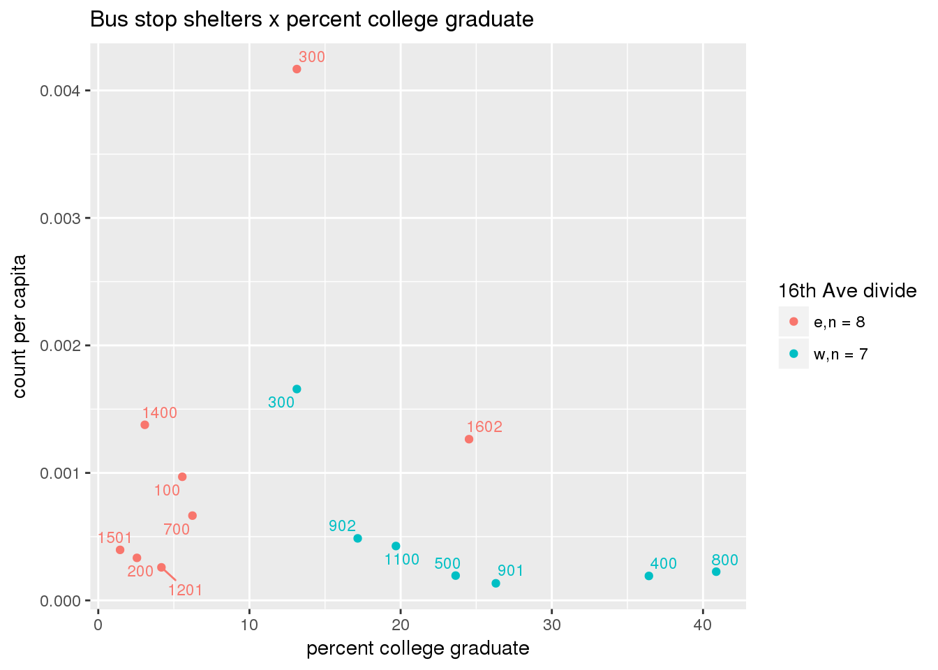
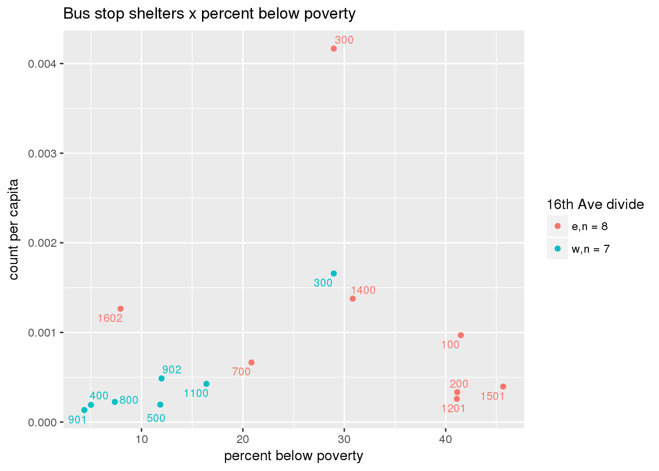
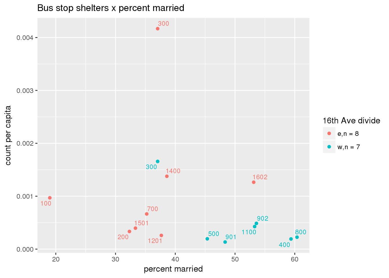
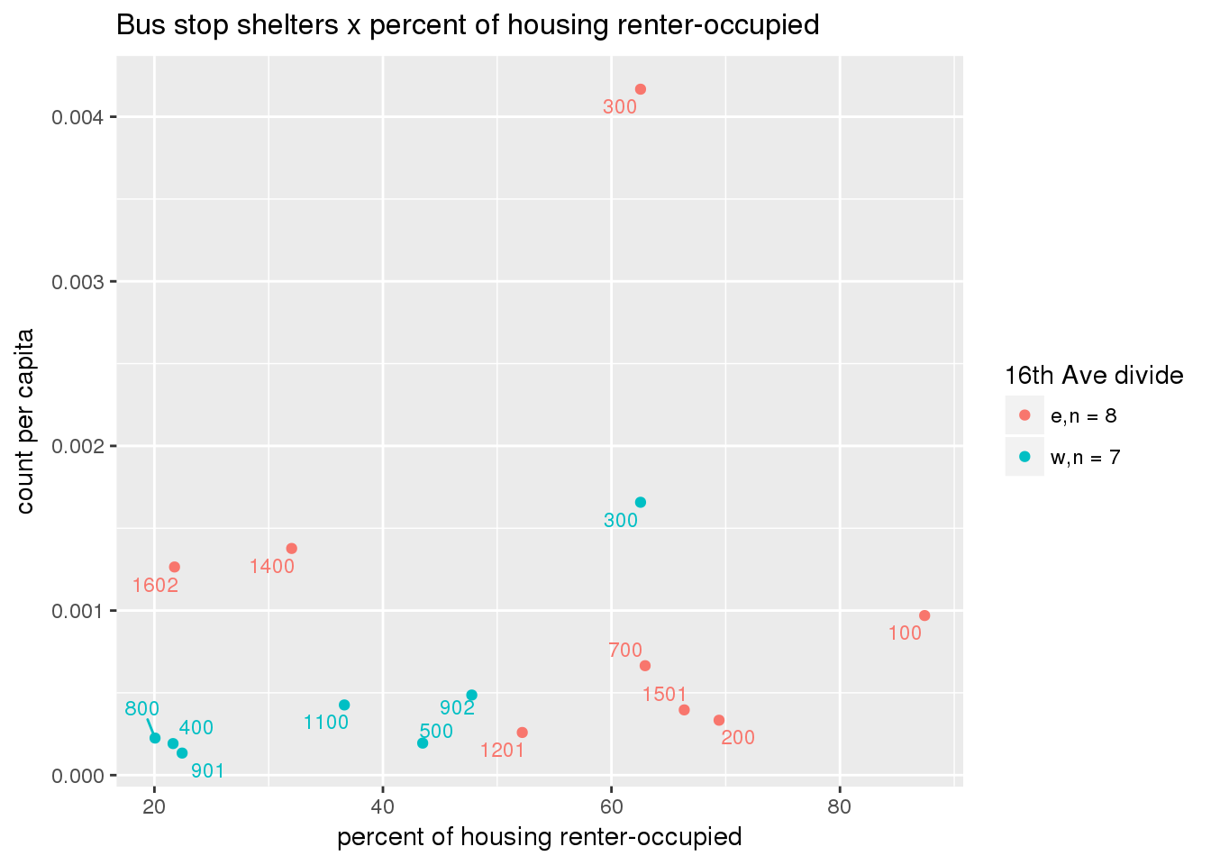
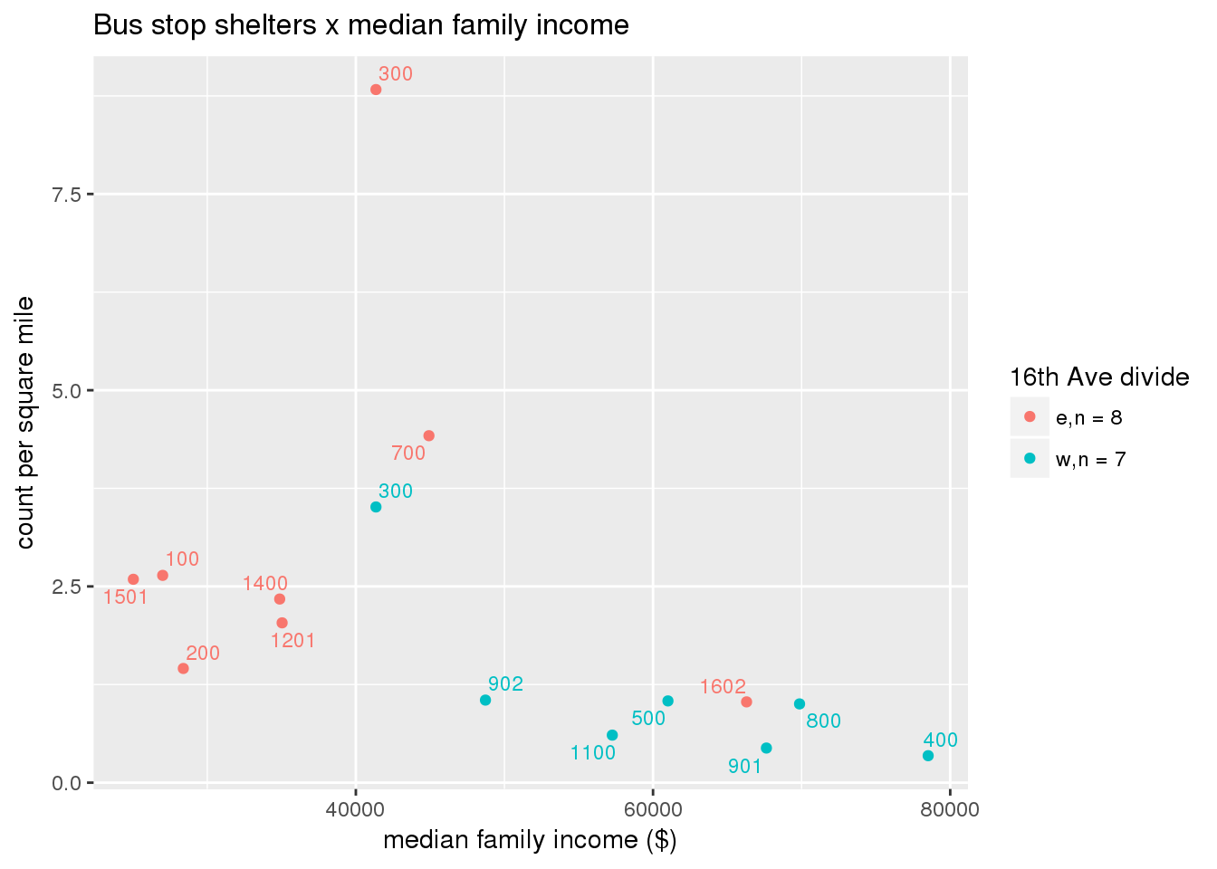
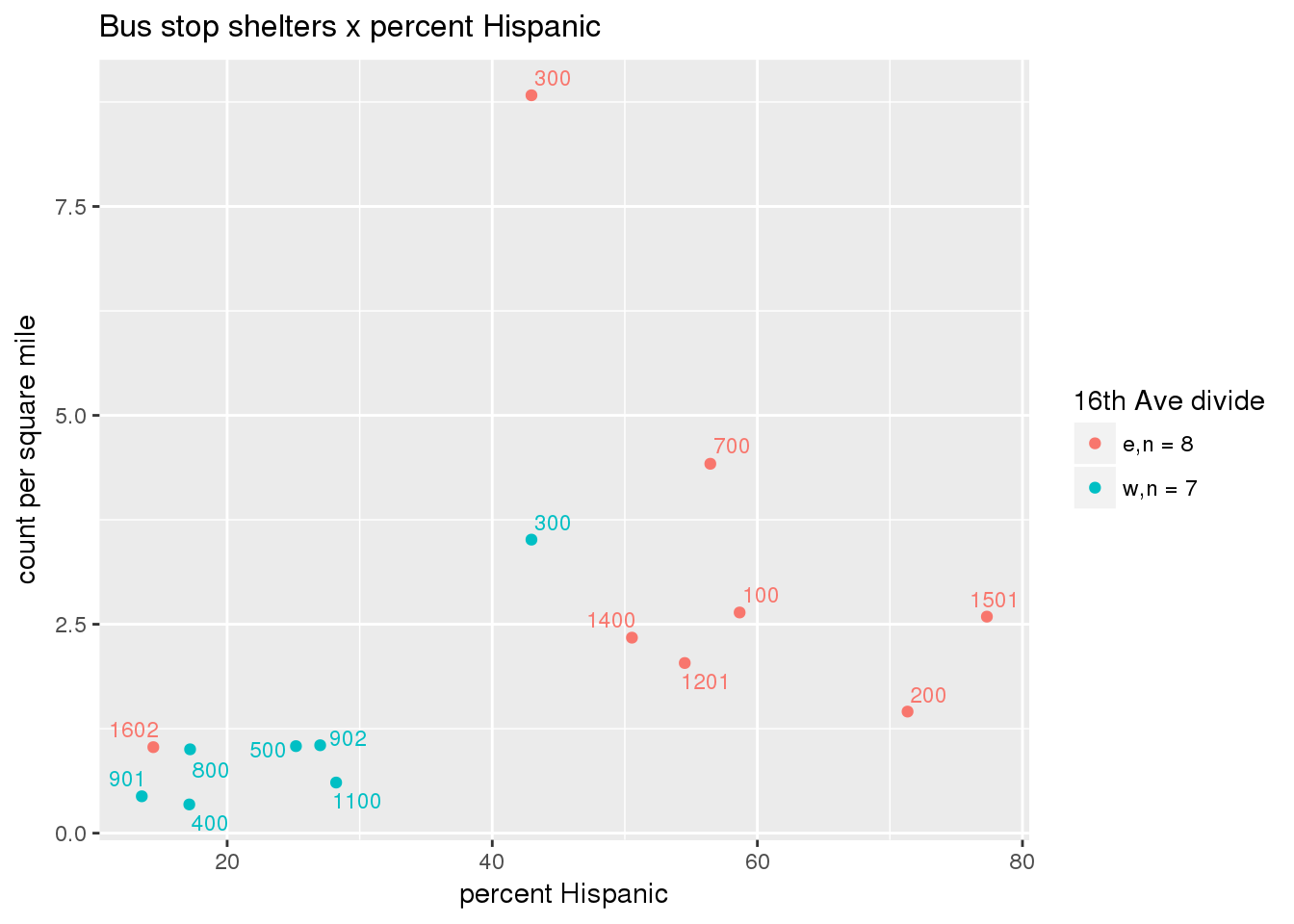
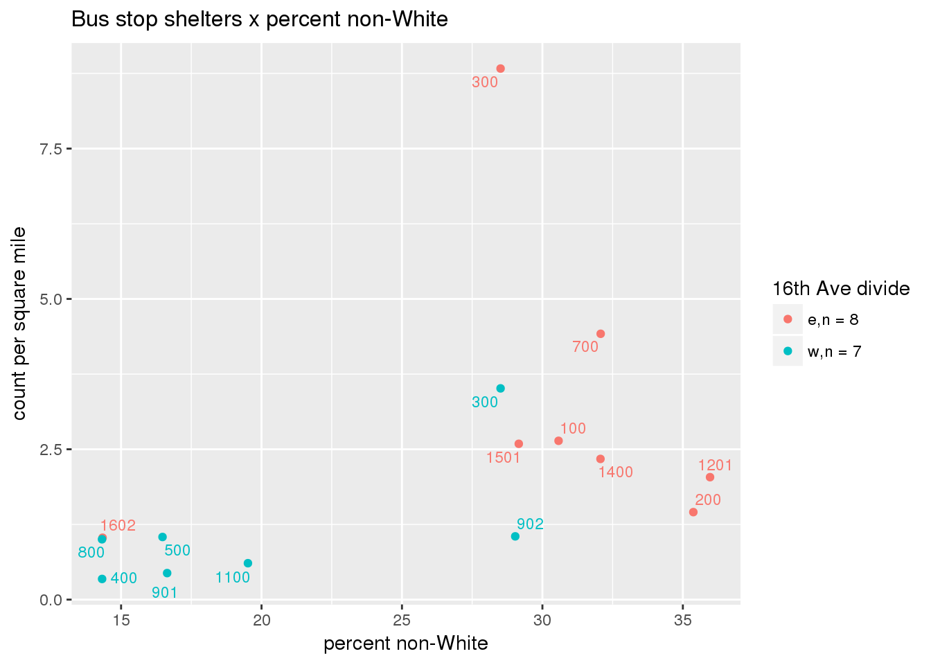
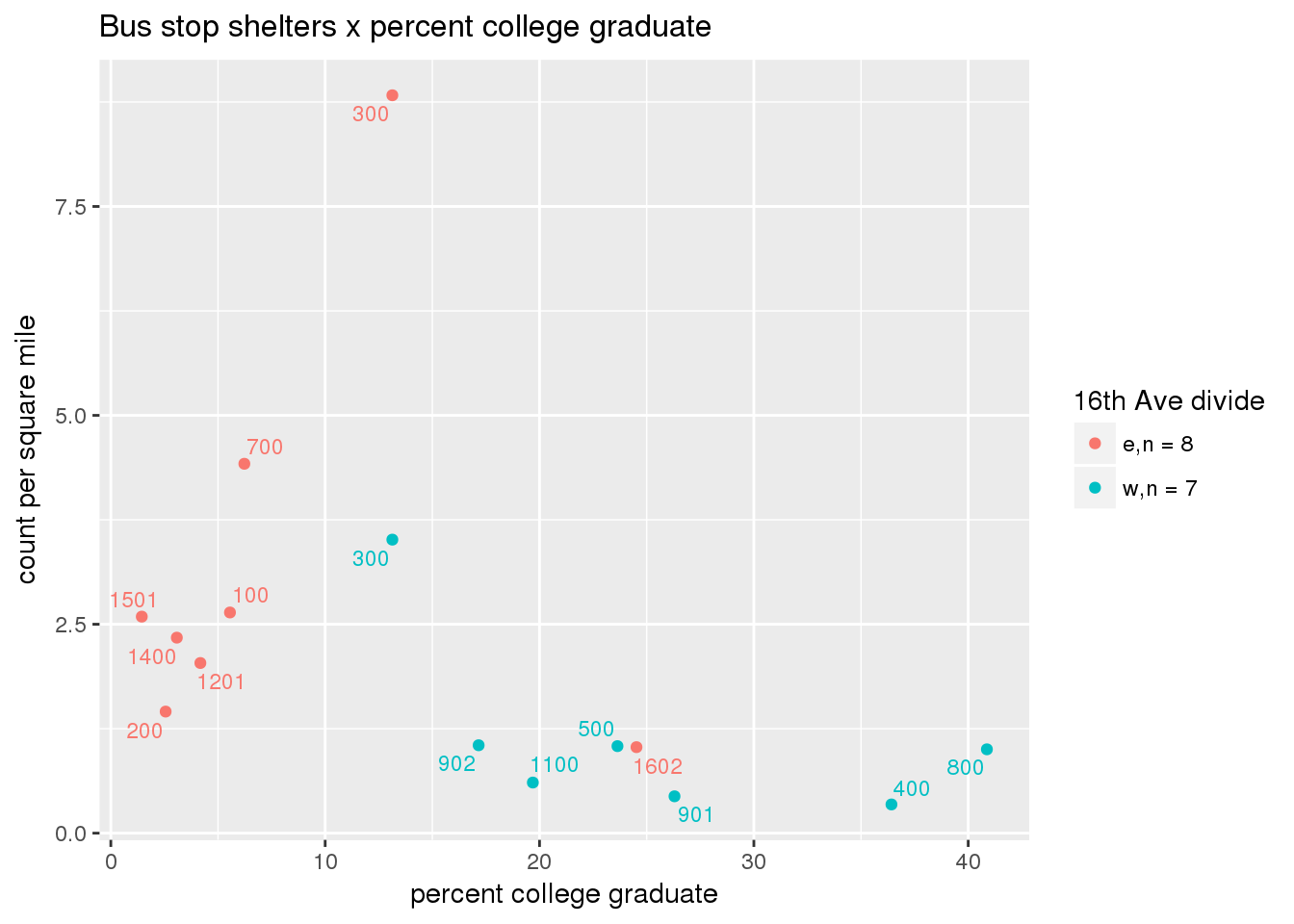
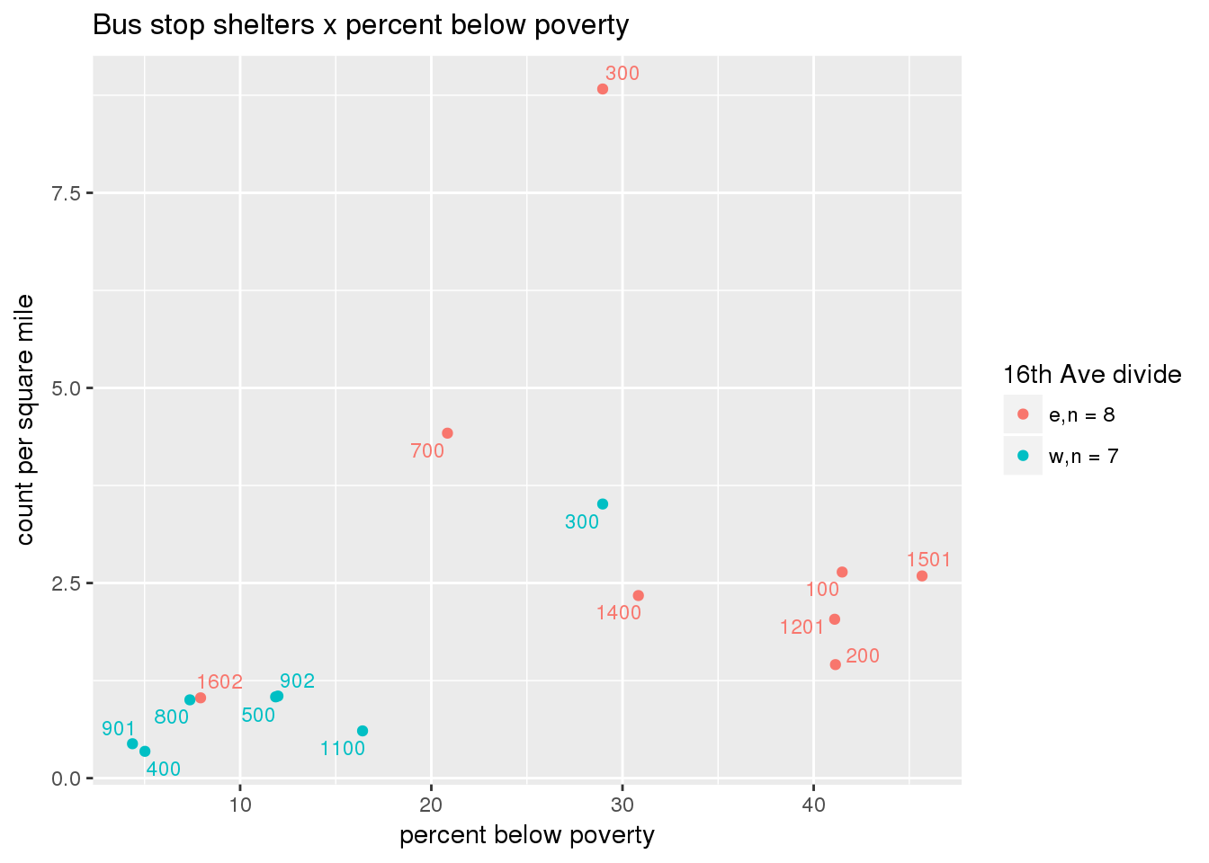
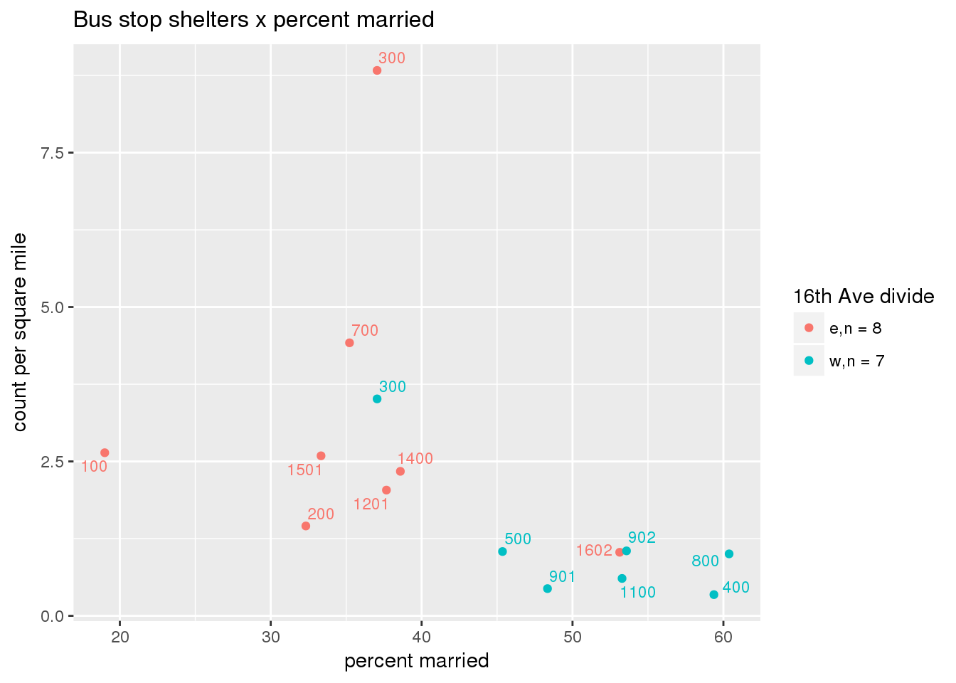
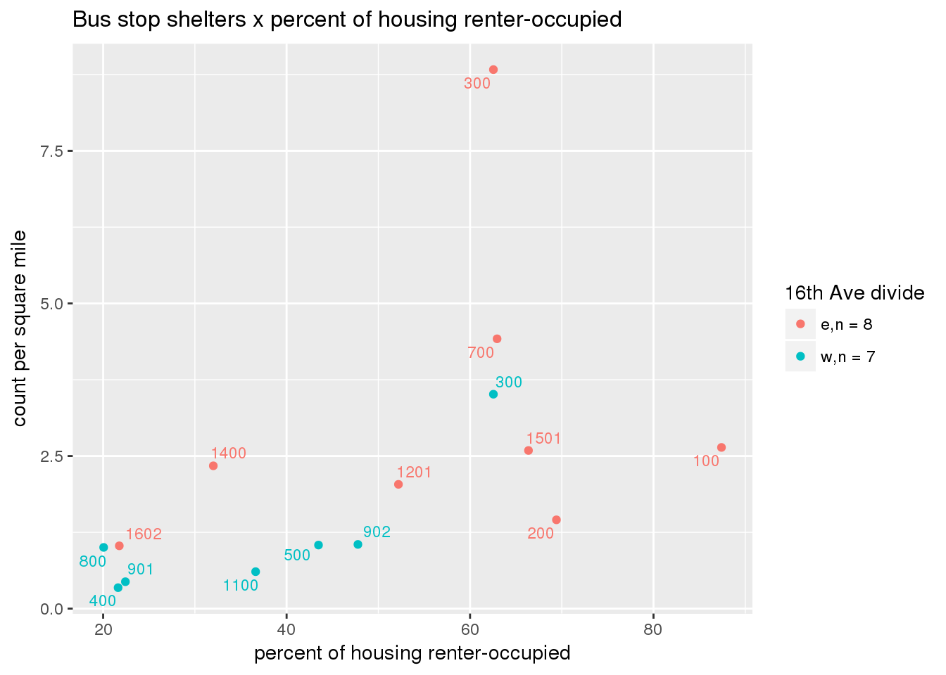
3.5.4.3 Shelters
Bus shelters per capita
busshelter <- ptfcn(pttablename = "busstops", where = "where shelter = 'Y'", normvar = "capita", mytitle = "Bus stop shelters", legend_title = "16th Ave divide")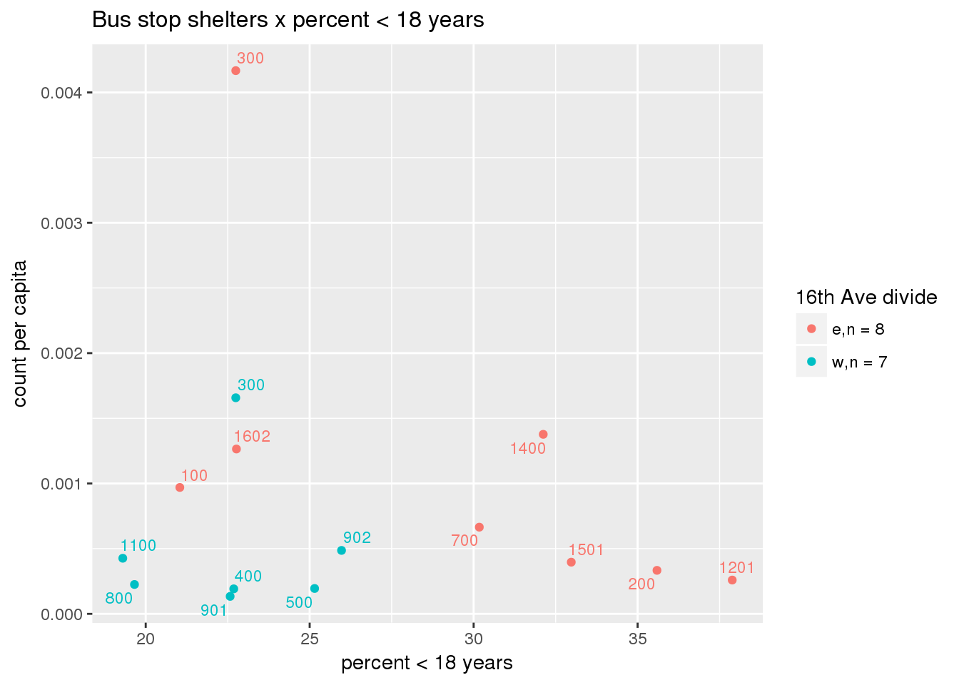
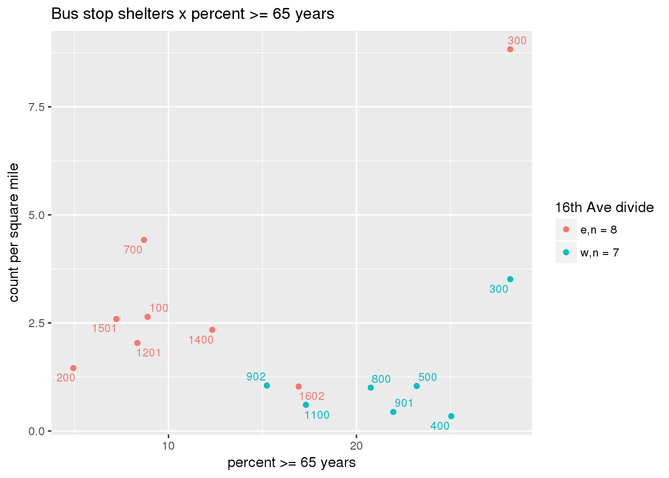
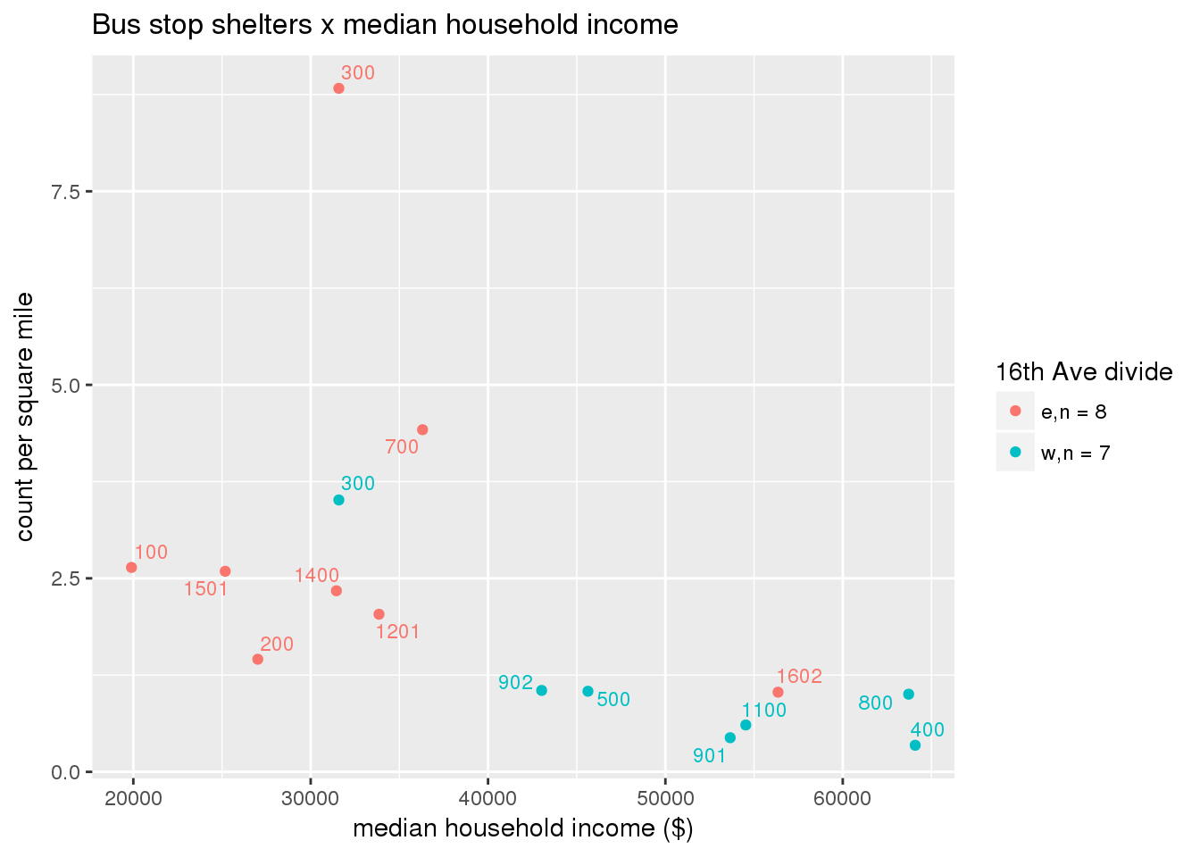
Bus shelters normalized by area
busshelter_norm <- ptfcn(pttablename = "busstops", where = "where shelter = 'Y'", normvar = "area", mytitle = "Bus stop shelters", legend_title = "16th Ave divide")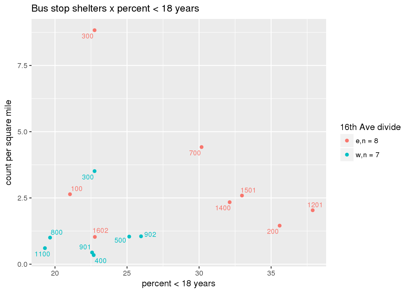
# zip the graphs
                                        system("cd /projects/yakima_equity/www/images; zip 00_all_images.zip *png *pdf")

                                        # pdf the graphs
                                        system("cd /projects/yakima_equity/www/images; convert *.png -quality 100 00_all_images.pdf")

                                        # zip the maps
                                        system("cd /projects/yakima_equity/www/maps; zip 00_all_maps.zip *.png")

                                        # PDF the maps
                                        system("cd /projects/yakima_equity/www/maps; convert *.png -quality 100 00_all_maps.pdf")
4 Downloads
Downloadable maps are available as a single PDF, or as a zip file.
Graphs are available as a single PDF or as a zip file.